When Should a Trial Stop?
Bayesian Adaptive Design in a Kenyan Eye Care Program
This note is a companion to the Experimental Designs chapter of Global Health Research in Practice. It uses a recent trial in Kenya to introduce Bayesian adaptive trial design—an approach that lets the data determine when a trial should stop, rather than fixing the sample size in advance.
The Eye Care Access Problem
In Meru County, Kenya, teams of screeners go door to door with smartphones, screening people’s vision using an app called Peek Acuity. Anyone with a possible eye problem is referred to a local treatment outreach clinic for further assessment and care. The service is free. But as of 2024, only about 46% of people referred after screening actually showed up.
The problem wasn’t evenly distributed. Allen et al. (2024) analyzed program data and found that younger adults (aged 18–44) were the group least likely to access care—only about a third attended, compared with over half of older adults. Age, gender, and occupation were all associated with access, but the gap was widest among younger adults.
So the researchers did something unusual. Instead of designing a traditional trial—writing a protocol, calculating a sample size, recruiting participants into a standalone study—they embedded a randomized trial directly inside the screening program’s software. The Peek Vision app already tracked every referral. They added code that randomly assigned each consenting patient to receive either the standard referral process or an enhanced version: a new counseling script delivered at the point of referral, plus an additional SMS reminder. The trial ran in the background of routine care, with randomization, data collection, and outcome assessment all automated.
And they didn’t decide in advance how many people to enroll. Instead, they used a Bayesian adaptive design with stopping rules that checked the accumulating data every 7 days. If the evidence was strong enough in either direction, the trial would stop.
It stopped after 30 days. With 879 younger adults enrolled, the posterior probability that the intervention group had higher attendance was 98.6%. The trial was over.
Why Not Just Run a Standard Trial?
In a conventional randomized trial, you start by specifying the effect size you want to detect, the statistical power you want (usually 80-90%), and the significance level (usually 5%). From these, you calculate a fixed sample size. You enroll that many participants (maybe inflated for expected attrition), collect the data, and then analyze the results. If you look at the data early and stop because the results look good, you inflate your Type I error rate. The whole framework depends on committing to the sample size in advance.
This approach has real strengths. The logic is straightforward, the error rates are well understood, and decades of regulatory practice are built around it. But it also has limitations, especially in the kind of pragmatic, service-delivery context this trial operated in.
First, you need to specify the effect size in advance. Allen et al. didn’t have a strong basis for this. They were testing a low-cost counseling modification co-designed with the community, embedded in an existing program. They didn’t know whether to expect a 2-percentage-point improvement or a 10-percentage-point improvement. The traditional approach would be to set a lower bound on what effect size would be clinically meaningful and go from there.
Second, a fixed-sample trial can waste resources. Frequentist designs do have a solution for this: group sequential methods allow pre-planned interim analyses at a small number of scheduled looks, with adjusted significance thresholds (like O’Brien-Fleming boundaries) to control the overall Type I error rate. But these require specifying the number and timing of interim looks in advance, and each look uses a stricter threshold to preserve error control. The Bayesian approach used here is different. It monitors data continuously, updating the posterior probability at every analysis point, without needing to adjust for multiple looks. The inferential framework handles repeated testing naturally.
Third, this trial was designed as one arm of a broader platform. The FAIR approach (Find cases, Analyze clinic data to identify non-attenders, Interview and survey to identify barriers and potential solutions, Randomize solutions to test their effectiveness) is meant to cycle through multiple service modifications over time. Waiting months for a fixed-sample trial to complete before testing the next idea defeats the purpose.
How Bayesian Stopping Rules Work
The trial used Bayesian methods to monitor the data continuously. Here’s the core idea.
In a frequentist framework, you ask: “If there were no true difference between groups, how often would I see data at least this extreme?” That’s a p-value. You don’t get to update your beliefs as data accumulate. You wait until the end for inference.
In a Bayesian framework, you ask a different question: “Given the data I’ve seen so far, what’s the probability that the intervention is better than control?” You start with a prior belief about the effect, update it with each batch of data, and get a posterior distribution that directly tells you the probability of any hypothesis you care about.
Priors, posteriors, and what the trial did
Bayesian analysis has three ingredients: a prior (what you believe before seeing data), a likelihood (what the data tell you), and a posterior (your updated belief after combining the two).
The prior is where this approach differs most from frequentist analysis. Before the trial starts, you express your uncertainty about the unknown quantity as a probability distribution—a curve that shows which values you consider plausible and how plausible each one is. As data come in, the prior gets updated into a posterior distribution that reflects both your starting beliefs and the evidence.
The posterior is the payoff. It’s not a single point estimate but a full distribution over the unknown quantity. From it, you can read off any summary you want: the most likely value, a credible interval (the Bayesian analog of a confidence interval), or, crucially for this trial, the probability that one group’s attendance rate is higher than the other’s. And because the posterior updates every time new data arrive, you can ask these questions repeatedly as the trial runs.
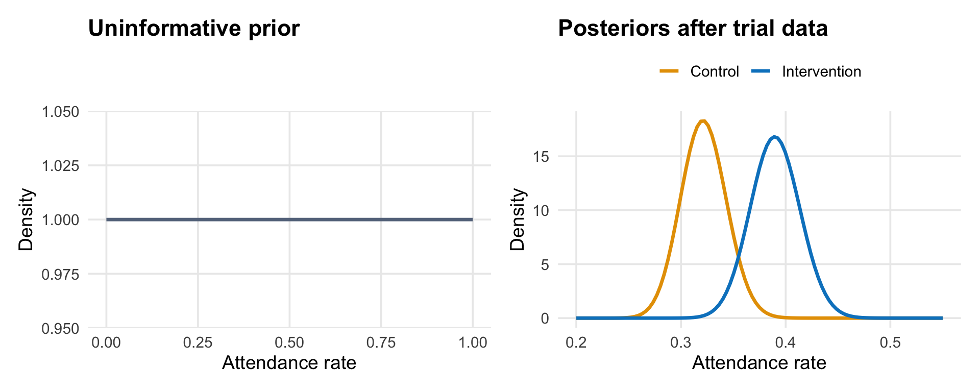
The figure below illustrates the logic. The left panel shows what a completely uninformative prior looks like: a flat line that assigns equal probability to every possible attendance rate.1 The right panel shows what happens after observing the trial data: the posteriors for each group are tightly concentrated around the observed rates, with the intervention posterior sitting to the right of the control posterior.
Allen et al. put their prior directly on the odds ratio between groups—the quantity that answers “how much better or worse is the intervention compared to control?” An odds ratio of 1.0 means no difference. Their prior was centered at 1.0 with a 95% credible interval from 1/30 to 30, which is extremely wide: it says the intervention could make things 30 times better or 30 times worse, and everything in between is roughly plausible.
Why such a wide prior? Because the prior is on the odds ratio—how much the intervention changes attendance relative to control—and the researchers had no strong basis for predicting that. They knew the baseline attendance rate was about 32%, but that doesn’t tell you how much an enhanced counseling script will shift it. A wide prior on the odds ratio is an honest reflection of that uncertainty: they let the data determine whether the intervention helped, rather than encoding a guess.2
The stopping rules
Every 7 days, the trial algorithm computed the posterior probability that the intervention group’s attendance rate was higher than the control group’s. Specifically, it used Monte Carlo simulations to generate the full posterior distribution of the difference between groups, then checked two rules:
Stopping for superiority: Is there a greater than 95% probability that one group is better (i.e., the difference is greater than 0%)? If so, declare that group superior and stop.
Stopping for equivalence: Is there a greater than 95% probability that the difference between groups is within ±1% of zero (i.e., negligible)? If so, declare equivalence and stop.
The first rule catches a clear winner. The second prevents the trial from running indefinitely when both arms perform the same.
Let’s simulate how this process works. Imagine the trial has just started. Patients are being enrolled one at a time, randomized to control or intervention, and I’m tracking whether each one accesses care within 14 days. The table below shows what the first 50 patients might look like, using simulated data with attendance rates similar to the actual trial (32% for control, 39% for intervention).
| Patients per arm | Attended | Rate | Attended | Rate |
|---|---|---|---|---|
| 5 | 3 | 60.0% | 1 | 20.0% |
| 10 | 4 | 40.0% | 3 | 30.0% |
| 15 | 5 | 33.3% | 5 | 33.3% |
| 20 | 7 | 35.0% | 9 | 45.0% |
| 25 | 10 | 40.0% | 12 | 48.0% |
Early on, the rates bounce around. With only 10 patients per arm, a single person attending or not can swing the rate by 10 percentage points. This is the noise the Bayesian framework has to see through. As more patients enroll, the cumulative rates stabilize, and the posterior distributions narrow.
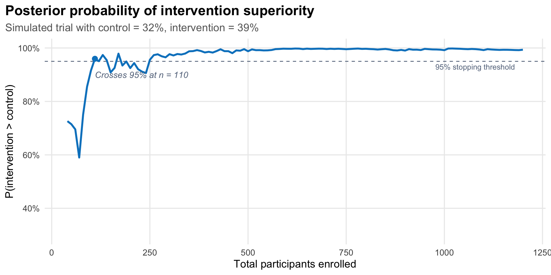
The figure below shows this process from the Bayesian perspective: at each point, I compute the posterior probability that the intervention group’s attendance rate is higher than the control group’s.
What did the trial actually find?
At the first analysis point—30 days after the trial began, with 879 younger adults enrolled—147 of 458 (32.1%) in the control group had accessed care, compared with 164 of 421 (39.0%) in the intervention group. The posterior probability of superiority was 98.6%, exceeding the 95% threshold. The trial stopped.
The mean effect difference was 6.4 percentage points (95% credible interval: 0.6 to 13.1). In a secondary analysis including all adults (aged 18–99), the posterior probability of superiority was 90.8%—notable but below the stopping threshold, suggesting the intervention’s benefit was concentrated among the younger adults it was designed for.
The trade-offs of adaptive stopping
This efficiency comes with trade-offs that Allen et al. are transparent about.
The first is a high false positive rate. Strictly speaking, Type I and Type II errors are frequentist concepts—they describe long-run error rates across hypothetical repetitions of the experiment, not something a Bayesian analysis directly targets. But it’s common practice to evaluate a Bayesian design’s frequentist operating characteristics: if you ran this stopping rule many times under the null hypothesis (no true difference), how often would it incorrectly declare superiority? Allen et al. did exactly this. Based on their Monte Carlo simulations, the trial had a 36.3% chance of declaring superiority when there was no true difference—far above the conventional 5%. This was a deliberate choice. The intervention was low-cost (an extra minute of counseling and an additional SMS reminder), the risks were negligible, and the research question was about rapid service improvement, not regulatory approval. In their words, “it is more important to avoid type II error than type I error” in this context.
The second trade-off is early stopping bias. Trials that stop early because results look promising tend to overestimate the treatment effect, because they’re more likely to stop at a random high point. Allen et al. acknowledge this: “there is a chance that the magnitude of difference between the groups is an overestimate because, on average, stopping rules end the trial at a local peak.” The control group rate of 32.1% matched the program’s historical baseline of 32%, which is reassuring, but the 6.4-percentage-point difference could be inflated.
The figure below illustrates why. I simulated 50 trials where the true difference between groups is 5 percentage points. Each grey line traces one trial’s observed effect as participants accumulate. The blue dots mark trials that crossed the 95% posterior probability threshold and stopped early. Notice they tend to sit above the dashed line (the true effect), because they stopped during a random upswing, locking in an inflated estimate. The orange dots on the right edge show trials that ran to 1,000 participants without triggering the stopping rule; their final estimates cluster much closer to the true effect.
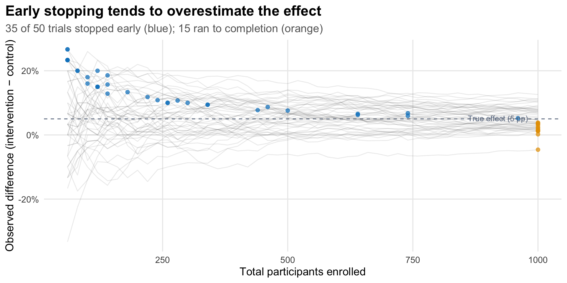
Notice that the orange dots also tend to sit slightly below the true effect, not centered on it. This isn’t a coincidence—it’s the other side of the same selection. Trials where random variation pushed the observed effect above average were more likely to trigger the stopping rule and exit early (blue dots). The trials that made it to full enrollment are the leftover ones where the effect was running below average, at least at the earlier sample sizes. Early stopping doesn’t just inflate the estimates of trials that stop—it also filters which trials make it to full enrollment.
Do these trade-offs make the trial’s conclusions unreliable? Not necessarily. They’re design choices appropriate to the context. A trial testing a new drug would need tighter error control. A trial testing whether slightly different wording in a counseling script improves attendance at a free eye clinic has different stakes. The researchers explicitly chose to prioritize avoiding Type II errors (missing a real improvement) over controlling Type I errors (incorrectly adopting an ineffective intervention), because the costs of adoption were negligible. The intervention was an extra minute of counseling and an additional SMS reminder—essentially free to add to the existing screening workflow. If it works even a little without adding cost or complexity, adopting it is a net win even if the effect size is overestimated.
That rationale doesn’t always generalize, however. For interventions that are expensive, risky, or resource-intensive to deliver, early stopping bias and inflated Type I error rates are much more consequential. The tolerance for these trade-offs should match the stakes of being wrong.
Tip
Reducing early stopping bias. Allen et al. chose aggressive settings—a flat prior, frequent checks (every 7 days), an early first look, and a 95% stopping threshold—because the stakes were low. When the stakes are higher, several design choices can reduce the risk of stopping prematurely on an inflated estimate:
- Delay the first look. Requiring a minimum sample size before the first interim analysis (e.g., 25–50% of the planned maximum) avoids checking when estimates are dominated by noise.
- Raise the stopping threshold. Requiring 99% posterior probability instead of 95% means the data have to be more convincing before the trial stops, reducing the chance of stopping during a random upswing.
- Use a skeptical prior. A prior centered on zero or a small effect slows the posterior’s movement toward the stopping boundary. The data have to overcome the prior’s skepticism, which acts as a brake on premature stopping.
- Check less frequently. Fewer interim looks means fewer opportunities to stop at a local peak. Checking monthly or at pre-specified enrollment fractions rather than weekly reduces this risk.
- Correct the estimate after stopping. Accept that the stopping rule introduces bias, but apply a bias-adjusted estimator (e.g., a median-unbiased estimate or shrinkage correction) when reporting the final result.
No single adjustment eliminates the problem, but combining several of these—a mildly skeptical prior, a delayed first look, and a higher threshold—can substantially reduce early stopping bias while preserving much of the efficiency advantage of adaptive designs.
Equity-Focused Design
One thing this trial does that’s worth noting briefly: it starts from the question of who isn’t being served, rather than what intervention might work in general.
Before running the trial, the researchers followed what they call the FAIR approach (Allen et al. 2025). They analyzed program data to find the demographic group with the lowest access rates (younger adults). They conducted 67 qualitative interviews with younger adults who hadn’t attended their appointments, asking what got in the way. They then surveyed 401 additional non-attenders and asked them to rank potential solutions. The top-ranked ideas were discussed in a workshop with stakeholders from the program, government, funders, and community, who agreed on a bundle of five counseling modifications to test.
The intervention wasn’t designed by researchers guessing at barriers. It was designed by the people who experienced them. The trial then tested whether this co-designed solution actually worked, using the adaptive methods described above.
Platform Trials
This trial was conducted as part of a broader adaptive platform trial. The idea behind a platform trial is that you don’t just test one intervention and stop. You build a standing trial infrastructure that can test multiple interventions sequentially—swapping in new arms as old ones are resolved.
In this case, the FAIR approach generated a ranked list of potential service modifications. The counseling bundle was first. Future iterations could test appointment scheduling changes, different referral pathways, or transport support, each using the same embedded, adaptive architecture, with the same Bayesian stopping rules.
This matters for how you think about evidence generation in health programs. Instead of a one-off study that takes years, you get a continuous cycle: identify the gap, design the fix, test it quickly, adopt or move on.
Take-Home Messages
Bayesian adaptive designs let data determine when a trial stops. Instead of fixing the sample size in advance, you monitor the posterior probability of your hypothesis as data accumulate and stop when the evidence is strong enough. This can be dramatically more efficient than traditional designs—but it requires accepting different trade-offs around error rates.
Embedding a trial inside an existing program changes what’s possible. When randomization, data collection, and outcome assessment are automated within service delivery software, trials can run faster, cheaper, and with fewer logistical barriers. The result is evidence about how interventions work in practice, not just under ideal conditions.
Error rate trade-offs should match the stakes. This trial accepted a 36% Type I error rate—unthinkable for a drug trial, but defensible for a low-cost service modification with negligible risks. The right level of statistical stringency depends on what you’re testing and what happens if you’re wrong.
Starting from equity gaps, not intervention ideas, changes what you build. The FAIR approach—finding who’s being left behind, interviewing them, co-designing solutions, then testing rigorously—produced an intervention that worked for its intended population. The intervention had negligible impact on older adults, who already had higher access rates. It was designed for the people it helped.
Footnotes
This is a Beta(1,1) distribution, the simplest uninformative prior for a proportion. Allen et al.’s actual prior was on the odds ratio, not on each group’s rate directly, but the intuition is the same: start wide open, let the data do the work.↩︎
A middle ground would be a weakly informative prior on the odds ratio—one that doesn’t predict the direction of the effect but rules out implausible extremes. For instance, a prior that concentrates most of its mass between odds ratios of 0.5 and 2.0 would say “the intervention probably doesn’t make things dramatically better or worse” while still allowing the data to dominate. This makes sense on substantive grounds: a modified counseling script was never going to double attendance or cut it in half. As the Stan development team’s prior choice recommendations put it, weakly informative priors “contain enough information to regularize” by ruling out unreasonable values while remaining flexible enough to let the data speak. In practice, with 879 participants, the data would overwhelm a weakly informative prior anyway—but the choice matters more in smaller trials or when the stopping rules are evaluated early, precisely the situation where adaptive designs operate.↩︎