This note is a companion to the Causal Inference chapter of Global Health Research in Practice, which introduces DAGs, the three causal structures, and effect identification. Here we apply those ideas to a real study.
Eric talks with Dr. Judith Lieber from the London School of Hygiene and Tropical Medicine about her new paper in the Lancet Global Health featured in this note.
The Study
An episiotomy is a surgical cut to the perineum—the tissue between the vagina and anus—made during the final stages of delivery. The idea is to create a controlled incision rather than risk an uncontrolled tear, particularly when delivery needs to happen quickly (fetal distress, shoulder dystocia) or when an instrument like forceps or vacuum is used. For decades, episiotomy was performed routinely on first-time mothers in many settings.
But the evidence caught up with the practice. Routine episiotomy doesn’t prevent severe tearing—it may actually increase it—and the incision itself is a wound that bleeds. WHO now recommends against routine use. Despite this, rates remain stubbornly high: over 80% of first-time mothers in Pakistan and over 60% in Nigeria received one in a recent trial. And here’s the concern that matters most in these settings: episiotomy may increase the risk of postpartum haemorrhage—the leading cause of maternal death worldwide, with nearly 90% of haemorrhage deaths occurring in south Asia and sub-Saharan Africa.
A 2026 study in The Lancet Global Health investigated this question: does episiotomy increase the risk of postpartum haemorrhage in women with anaemia? The study was a cohort analysis nested within the WOMAN-2 trial—a large randomized trial of tranexamic acid for haemorrhage prevention that recruited over 15,000 women with moderate or severe anaemia across 34 hospitals in Nigeria, Pakistan, Tanzania, and Zambia.1
The researchers couldn’t randomize women to receive an episiotomy or not. The trial randomized a different treatment (tranexamic acid), so for the episiotomy question this was effectively an observational study—and that makes causal inference hard. They needed a way to think through the confounding problem before choosing their analysis strategy.
They used a directed acyclic graph. Let’s see why.2
The Problem: Why a Naive Comparison Fails
Imagine simply comparing haemorrhage rates between women who received an episiotomy and those who didn’t. If the episiotomy group bleeds more, the procedure must cause bleeding—right?
Not so fast. Women who receive episiotomies are not a random sample. They’re more likely to have experienced obstructed labour, instrumental delivery, or fetal distress—conditions that independently increase the risk of postpartum haemorrhage. A naive comparison confounds the effect of the procedure with the reasons it was performed.
So we need to adjust for confounders. But which ones? And how do we know we’re not accidentally adjusting for something we shouldn’t? This is where the DAG comes in.
A Quick DAG Primer
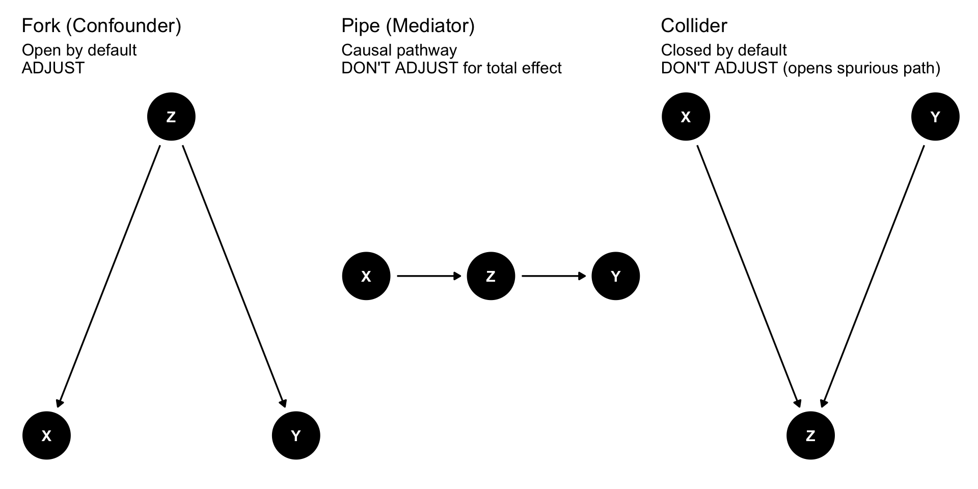
A directed acyclic graph (DAG) is a visual map of your causal assumptions. Nodes represent variables; arrows represent causal relationships. Every DAG, no matter how complex, is built from three basic structures. (For a fuller introduction, see the Causal Inference chapter.)
Show code
# Forkfork_dag <-dagify( X ~ Z, Y ~ Z,coords =list(x =c(X =0, Z =1, Y =2), y =c(X =0, Z =0.6, Y =0)))p_fork <-ggdag(fork_dag) +theme_dag() +labs(title ="Fork (Confounder)",subtitle ="Open by default\nADJUST")# Pipepipe_dag <-dagify( Z ~ X, Y ~ Z,coords =list(x =c(X =0, Z =1, Y =2), y =c(X =0, Z =0, Y =0)))p_pipe <-ggdag(pipe_dag) +theme_dag() +labs(title ="Pipe (Mediator)",subtitle ="Causal pathway\nDON'T ADJUST for total effect")# Collidercollider_dag <-dagify( Z ~ X + Y,coords =list(x =c(X =0, Z =1, Y =2), y =c(X =0.6, Z =0, Y =0.6)))p_collider <-ggdag(collider_dag) +theme_dag() +labs(title ="Collider",subtitle ="Closed by default\nDON'T ADJUST (opens spurious path)")p_fork + p_pipe + p_collider
Structure
Example in This Study’s DAG
Default
What to Do
Fork
Slow/obstructed labour → Episiotomy, Slow/obstructed labour → Spontaneous perineal tears → Postpartum haemorrhage
Open (biasing)
Adjust to close
Pipe
Episiotomy → Total perineal tears → Postpartum haemorrhage
Open (causal)
Don’t adjust for total effect
Collider
Episiotomy → Shorter labour ← Instrumental delivery
Closed (harmless)
Don’t adjust (opens bias)
Three structures, three rules. These are the building blocks you need to read any DAG.
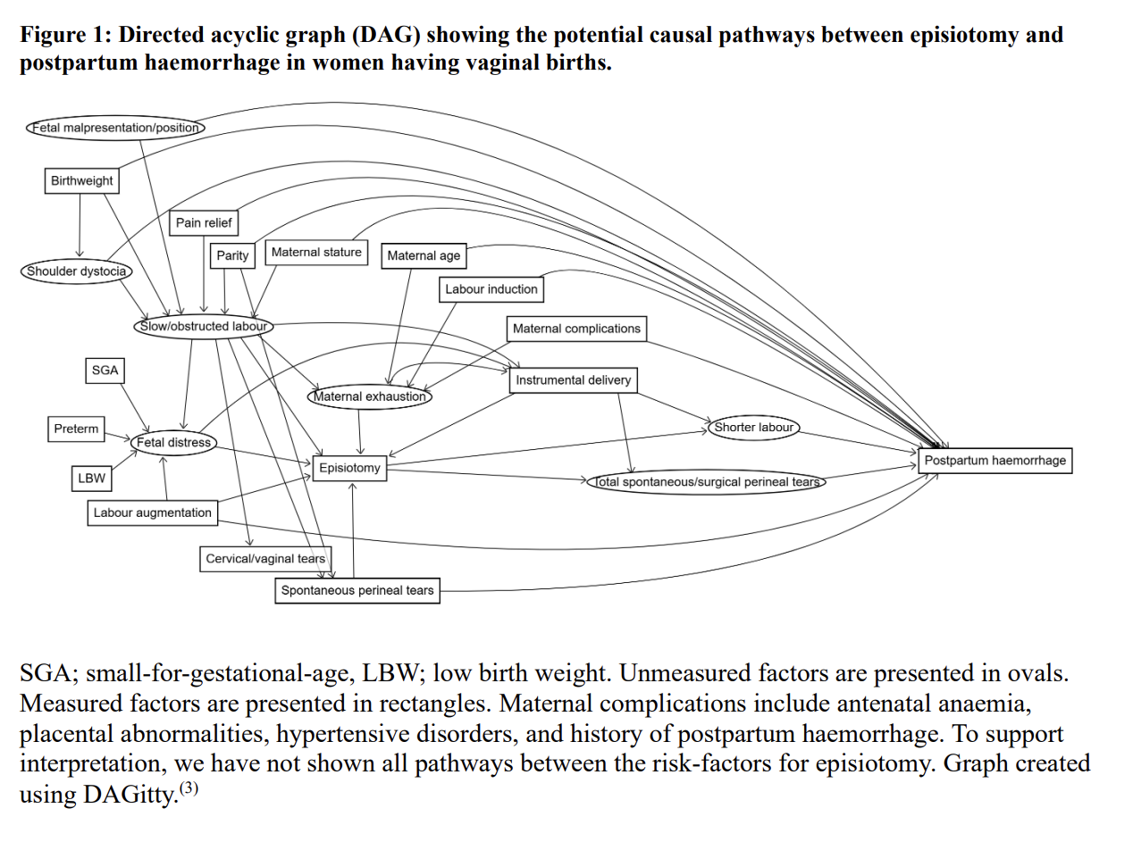
The Study’s DAG
The Lancet study authors built a DAG with over 20 variables. Their DAG distinguished between measured variables (shown as rectangles) and unmeasured variables (shown as ovals)—a critical distinction we’ll return to shortly.
Figure 1: DAG showing the potential causal pathways between episiotomy and postpartum haemorrhage in women having vaginal births. Unmeasured factors are presented in ovals; measured factors in rectangles. Source: Woodd et al. (2026), The Lancet Global Health, Appendix 6.
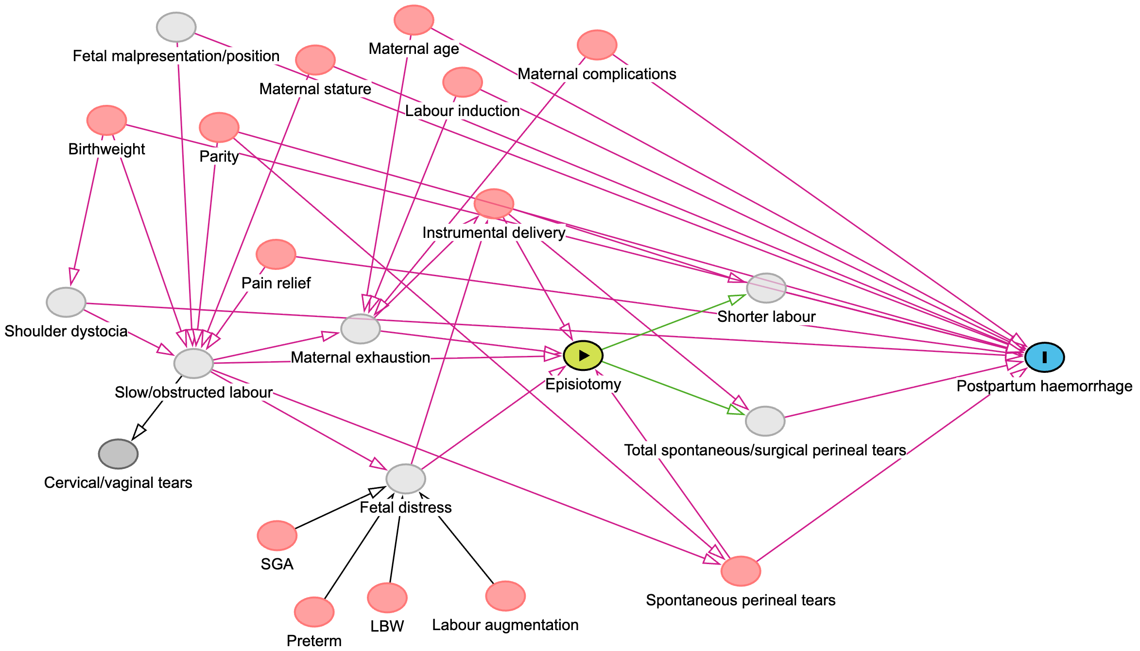
To analyze this DAG programmatically, I recreated it in DAGitty, a free tool for creating and analyzing causal diagrams (Figure 2). DAGitty color-codes the graph:
the green node is the exposure, episiotomy;
the blue node is the outcome, postpartum haemorrhage;
red nodes are ancestors of the exposure and the outcome (confounding);
light grey nodes are unmeasured (meaning they had no data on these variables); and
the dark grey node is another variable unrelated to exposure and outcome.
Figure 2: The authors’ DAG recreated in DAGitty, which identifies causal paths (green), other relationships (pink), and nodes on the causal pathway (blue).
We can load the same DAG into R to analyze it programmatically:
This is complex, but it’s still built from the same three structures. One thing to notice right away: the authors did not draw a direct arrow from episiotomy to postpartum haemorrhage. Every causal path is mediated—running through total perineal tears or shorter labour. This reflects a specific clinical assumption: episiotomy affects haemorrhage risk through these intermediate mechanisms, not independently of them. Let’s read the rest of the DAG:
Forks (confounders): Slow/obstructed labour causes both episiotomy and postpartum haemorrhage (through several pathways). Maternal exhaustion, fetal distress, and instrumental delivery also sit on backdoor paths. These need to be closed.
Pipes (mediators): Episiotomy → Total perineal tears → Postpartum haemorrhage. This is part of the causal effect. Adjusting for tears would block the pathway we’re trying to measure. The same goes for Episiotomy → Shorter labour → Postpartum haemorrhage.
Unmeasured variables (marked as latent in the DAG code): Shoulder dystocia, slow/obstructed labour, fetal distress, maternal exhaustion, fetal malpresentation, shorter labour, and total perineal tears are all unmeasured. If any of these sit on an open backdoor path, statistical adjustment can’t fully close it.
How the DAG Guided the Analysis
Counting the Paths
Once the DAG was drawn, the dagitty R package (or the DAGitty web tool) can enumerate every path connecting the exposure to the outcome.
Show code
# Enumerate all paths from episiotomy to postpartum haemorrhageall_paths <-paths(epis_dag)n_total <-length(all_paths$paths)n_open <-sum(all_paths$open)n_closed <- n_total - n_opencat("Total paths from Episiotomy to Postpartum haemorrhage:", n_total, "\n")
Total paths from Episiotomy to Postpartum haemorrhage: 100
Show code
cat(" Open paths:", n_open, "\n")
Open paths: 20
Show code
cat(" Closed paths:", n_closed, "\n")
Closed paths: 80
That’s 100 paths connecting episiotomy to postpartum haemorrhage. We can set aside the 80 closed paths for now—they’re already blocked and not causing any problems. (We’ll come back to why they’re closed and why it matters later.)
The 20 open paths are where the action is, and they fall into two categories:
Causal paths flow forward from episiotomy through mediators like total perineal tears or shorter labour to postpartum haemorrhage. These are the paths we want to remain open—they represent the effect we’re trying to measure.
Backdoor paths flow through confounders like slow/obstructed labour or fetal distress. These create bias—a spurious association between episiotomy and postpartum haemorrhage that has nothing to do with the causal effect. We need to close these paths through adjustment.
So the critical question becomes: what’s the minimum set of variables we need to adjust for to close all the biasing backdoor paths without blocking the causal ones?
The Minimal Adjustment Set
This is exactly what dagitty can calculate. It identifies the minimal sufficient adjustment set—the smallest set of variables that, if adjusted for, closes every backdoor path while leaving the causal paths intact.
Show code
# With latent (unmeasured) variables declared, dagitty only returns# adjustment sets composed of measured variablesadj <-adjustmentSets(epis_dag, type ="minimal")if (length(adj) ==0) {cat("No sufficient adjustment set exists using measured variables alone.\n\n")cat("This means the unmeasured confounders in the DAG sit on backdoor\n")cat("paths that cannot be closed through statistical adjustment.\n")} else {cat("Minimal sufficient adjustment sets:\n\n")for (i inseq_along(adj)) {cat(paste0(" Option ", i, ": { ", paste(adj[[i]], collapse =", "), " }\n")) }}
No sufficient adjustment set exists using measured variables alone.

This means the unmeasured confounders in the DAG sit on backdoor
paths that cannot be closed through statistical adjustment.
The DAG is telling us something important: there is no set of measured variables that fully closes all backdoor paths. Unmeasured confounders like shoulder dystocia, slow/obstructed labour, and maternal exhaustion sit on open backdoor paths, and because they weren’t measured in this study, no statistical adjustment can close them completely.
If we remove the unmeasured variable tags and ask dagitty what we would need to adjust for in an ideal world where everything was measurable:
Show code
# What if we could measure everything?epis_dag_all <- epis_daglatents(epis_dag_all) <-c()adj_all <-adjustmentSets(epis_dag_all, type ="minimal")cat("If all variables were measurable, minimal adjustment sets would be:\n\n")
If all variables were measurable, minimal adjustment sets would be:
Show code
for (i inseq_along(adj_all)) {cat(paste0(" Option ", i, ": { ", paste(adj_all[[i]], collapse =", "), " }\n"))}
This is the tension at the heart of the study. The DAG tells us what we need to adjust for, but some of those variables weren’t measured. The study authors were transparent about this. They adjusted for every measured confounder they could—sociodemographics, pregnancy history, maternal complications, birth characteristics, and country—and then conducted a quantitative bias analysis to assess how much unmeasured confounding (particularly by shoulder dystocia) could have distorted their results. Their conclusion: the findings were robust to this source of bias, but “bias from other unmeasured confounders remains possible.”
The DAG didn’t hand the authors a perfect solution. It told them what they should do based on their causal model—which confounders they could adjust for, which they couldn’t, and how to quantify the residual uncertainty. Compare this to the HPV vaccination example from the textbook, where the DAG revealed that unmeasurable confounders made confounder control essentially impossible—and pointed researchers toward a design-based solution (regression discontinuity) instead.
Closing the Paths They Could Close
With the measured confounders identified, the study authors used inverse probability of treatment weighting (IPTW)—a propensity score approach—to close the backdoor paths they could reach. Here’s the logic:
Estimate the propensity score: Use logistic regression to predict the probability of receiving an episiotomy based on the measured confounders identified by the DAG.
Calculate weights: Weight each woman by the inverse of her probability of receiving the treatment she actually got. This creates a “pseudo-population” where the measured confounders are balanced across groups.
Assess balance: Check that the weighting worked—that confounders are balanced between the episiotomy and no-episiotomy groups after weighting (absolute standardised mean differences < 0.10).
Estimate the effect: Fit the outcome model using the weights, with a random effect for hospital to account for clustering.
NotePropensity scores aren’t the only option
Once the DAG identifies which variables to adjust for, there are several ways to actually do the adjustment: multivariable regression, propensity score matching, stratification on the propensity score, or IPTW. The study authors chose IPTW because it handles many confounders flexibly and cleanly separates the design step (balancing confounders) from the analysis step (estimating the effect). The DAG tells you what to adjust for; the statistical method determines how.
The Results
After adjustment via IPTW, the study found that episiotomy was associated with a 1.88-fold increase in clinically diagnosed postpartum haemorrhage (95% CI: 1.33–2.66) and a 1.63-fold increase in calculated postpartum haemorrhage (95% CI: 1.14–2.34). The result was consistent across multiple sensitivity analyses.
Why You Can’t Just “Control for Everything”
A common instinct is to throw every available variable into the model and “control for everything.” The DAG shows why this can go wrong in two fundamentally different ways.
1. Adjusting for mediators blocks part of the effect. Notice what’s not in any valid adjustment set above: total perineal tears and shorter labour. These variables lie on the causal pathway from episiotomy to postpartum haemorrhage—they’re pipes, not forks. If we adjust for them, we block part of the very effect we’re trying to measure. Instead of estimating the total effect of episiotomy, we’d be estimating something closer to a direct effect—the portion not operating through tearing or labour duration.
The authors explicitly recognized this, noting that labour duration could be on the causal pathway and therefore should not be adjusted for. They estimated that roughly 40% of postpartum haemorrhage cases in women with episiotomy were attributed to tearing.3 Had they included tears as a covariate, they would have blocked this pathway and underestimated the total effect.
The principle: do not adjust for variables that sit downstream of your exposure if your goal is the total effect.
2. Adjusting for colliders creates bias where none existed. Remember the 80 closed paths we set aside earlier? They’re closed because each one passes through at least one collider—a variable where arrows point in from two or more directions along the path.4
Consider the path:
Episiotomy → Shorter labour ← Instrumental delivery → Total perineal tears → Postpartum haemorrhage
At Shorter labour, arrows point in from both sides. That makes it a collider. Colliders block paths by default, so this route is closed in the full DAG.
Now suppose we adjust for labour duration—perhaps by restricting the analysis to women with similarly short labours.
Shorter labour is caused by both episiotomy and instrumental delivery. Once we fix labour duration, learning about one cause tells us something about the other. If a woman had a short labour and did not have an episiotomy, instrumental delivery becomes a more likely explanation.
By conditioning on a shared effect, we create an association between its causes—even if they were unrelated in the full population. That induced association opens a backdoor path to haemorrhage.
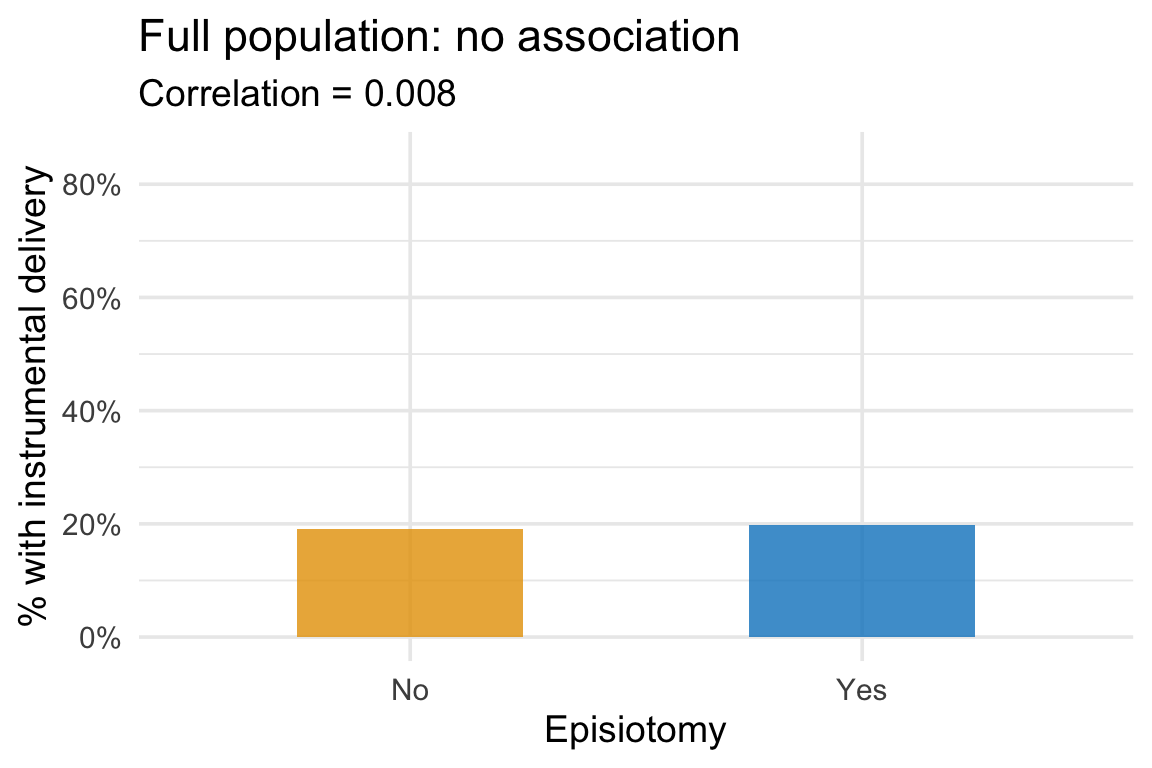
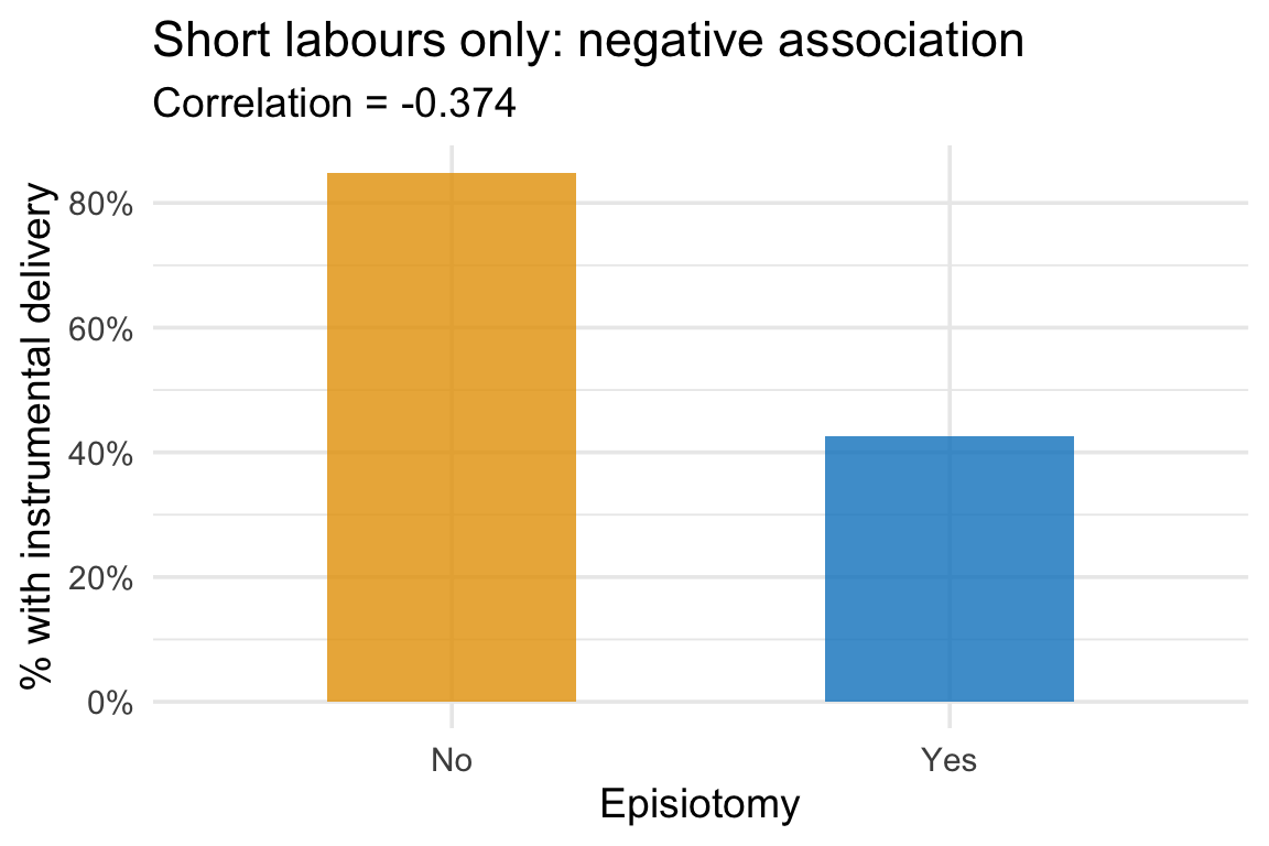
Let’s see this with a simple simulation. We’ll generate 5,000 women where episiotomy and instrumental delivery are completely independent—neither causes the other. But both shorten labour.
Show code
# Simulate independent causes of a shared effectset.seed(42)n <-5000sim <-tibble(episiotomy =rbinom(n, 1, 0.4),instrumental =rbinom(n, 1, 0.2),# Both reduce labour durationlabour_hours =12-3* episiotomy -4* instrumental +rnorm(n, 0, 2)) %>%mutate(short_labour = labour_hours <8,Episiotomy =ifelse(episiotomy ==1, "Yes", "No"),`Instrumental delivery`=ifelse(instrumental ==1, "Yes", "No") )
In the full population, the rate of instrumental delivery is the same regardless of whether a woman had an episiotomy—exactly what we’d expect from two independent variables:
Among women with short labours, those who did not have an episiotomy were more likely to have had an instrumental delivery. Conditioning on the shared effect created an association between its causes that did not exist in the full population.
We have potentially introduced bias by adjustment. If instrumental delivery also affects haemorrhage (as in our DAG), this induced association will bias the estimated effect of episiotomy.
The mistake feels reasonable—labour duration looks like a baseline characteristic. But in the DAG, it is downstream of the exposure. A harmless closed path becomes a new source of bias.
This is why “control for everything” is dangerous. Without a DAG, you might adjust for a mediator (blocking part of the effect) or a collider (creating bias from a path that was previously closed). The DAG tells you what to adjust for—and just as importantly, what not to.
TipThree rules for adjustment
Adjust for common causes of the exposure and outcome (confounders).
Do not adjust for mediators if you want the total effect.
Do not adjust for colliders.
Take-Home Messages
A DAG is a map of your assumptions. The study authors didn’t just “control for confounders.” They drew a DAG with 20+ variables, published it, and let readers evaluate their causal reasoning. Drawing your assumptions is the first step of any credible observational analysis.
The DAG tells you what to adjust for—and what not to. The minimum sufficient adjustment set closes all backdoor paths without blocking causal ones. Adjusting for a mediator blocks the effect you’re trying to measure. Adjusting for a collider creates bias where none existed.
Unmeasured confounding will happen. If a confounder on a backdoor path can’t be measured, statistical adjustment alone can’t fully identify the causal effect. The study authors used quantitative bias analysis to assess this limitation honestly. A DAG that includes unmeasured variables is more honest than one that pretends they don’t exist.
Every analysis has a DAG—whether you draw one or not. When you choose which covariates to “control for,” you’re implicitly making causal assumptions. A DAG makes them visible and debatable. Drawing one is always better than not.
Footnotes
The WOMAN-2 trial randomized women to tranexamic acid vs. placebo for postpartum haemorrhage prevention. The episiotomy question was not part of the trial’s experimental design—it was an observational analysis using the trial’s rich baseline and outcome data.↩︎
This was estimated as a population attributable fraction—the proportion of haemorrhage cases in the episiotomy group that would not have occurred absent tearing.↩︎
Forks and pipes are open by default. The only structure that’s closed by default is a collider. So when no conditioning has been applied, every closed path must contain at least one collider that blocks it.↩︎
Subsetting to short labours is equivalent to adjusting for labour duration in a regression model.↩︎