Chapter 12 · Video 5
Controlling confounding in observational data
Print layout
Slide 1


Controlling confounding in observational data
Slide 2
Confounder control is the strategy this chapter takes
A confounder is associated with both the exposure and the outcome
It creates a spurious association between them
Slide 3
Design phase
Design-phase strategies differ by design
Cross-sectional: limited control, beyond sampling for variation in confounders
Case-control: matching cases and controls on potential confounders
Cohort: restriction to a narrow range, or matching unexposed to exposed
Slide 4
Siddique et al., 2011
Outdoor air pollution and children's respiratory health in Delhi
Did outdoor air pollution affect children's respiratory health?
Children from different backgrounds differ in exposure and in baseline risk
Slide 5
Background affects both exposure and outcome
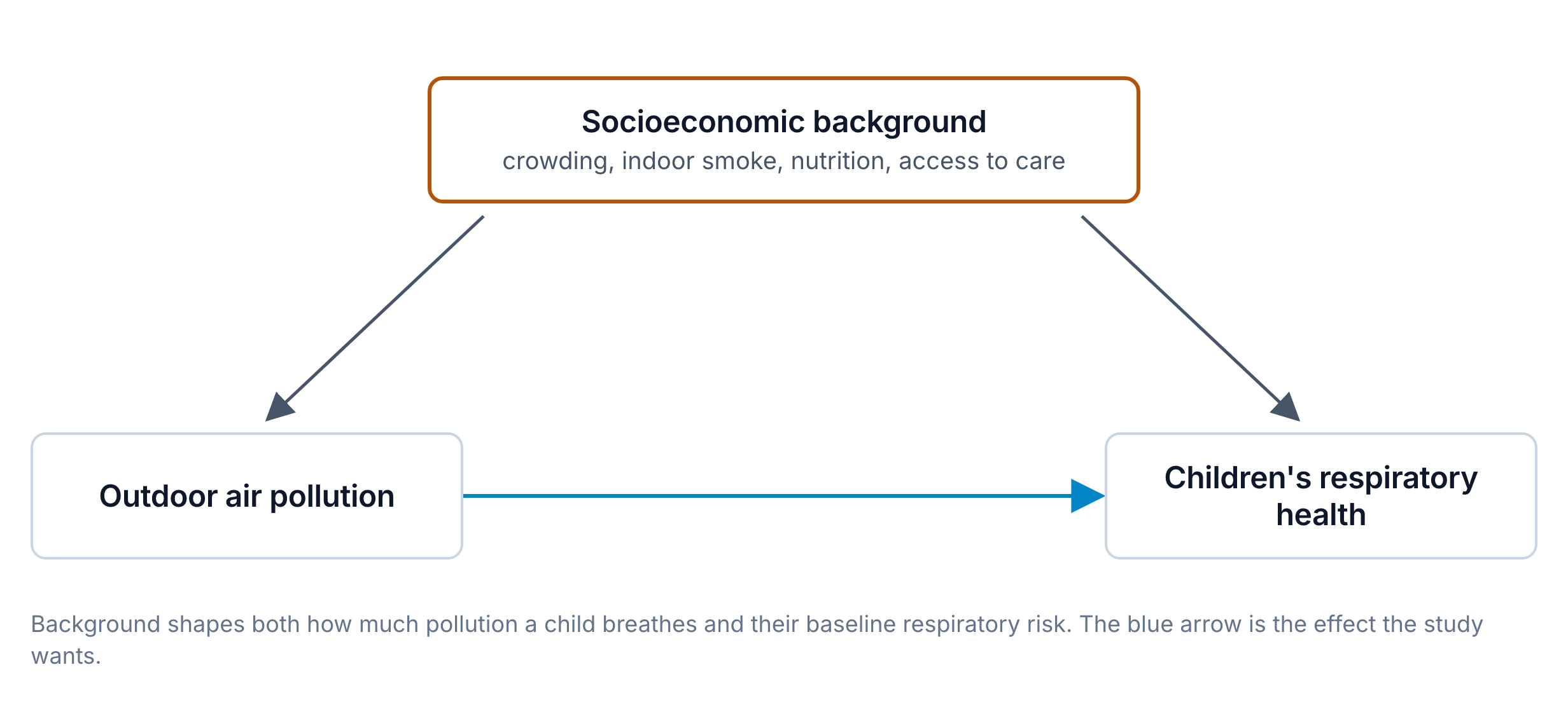
Socioeconomic background as a confounder of pollution and respiratory health, as the chapter describes the Delhi study.
Slide 6
Siddique et al., 2011
Matching before the analysis, regression during it
Matched on age, sex, parental education, household income, and neighborhood
Then multivariate logistic regression for further adjustment
Slide 7
Analysis phase
Stratification and multivariable regression ask different questions
Stratification
Present within each stratum?
Transparent, but only a few confounders
Multivariable regression
What is the association after adjustment?
Many confounders at once
Slide 8
Assimon et al., 2021
A propensity score models the probability of exposure
Each person's probability of being exposed, given their characteristics
Then match, stratify, or weight on that single score
Slide 9
Assimon et al., 2021
Why condense many confounders into one score
Regression with many confounders can become unstable in modest samples
One number makes matching and balance checks more straightforward
Slide 10
Target trial emulation
Approximating the conditions of a randomized experiment
No statistical method can fully substitute for randomization
Unmeasured confounding remains a fundamental limitation
Slide 11
IPTW
Inverse probability of treatment weighting creates a pseudo-population
Exposure becomes independent of measured confounders
The sample is reweighted to mimic random assignment
Slide 12
Weighted by the inverse probability of the treatment received
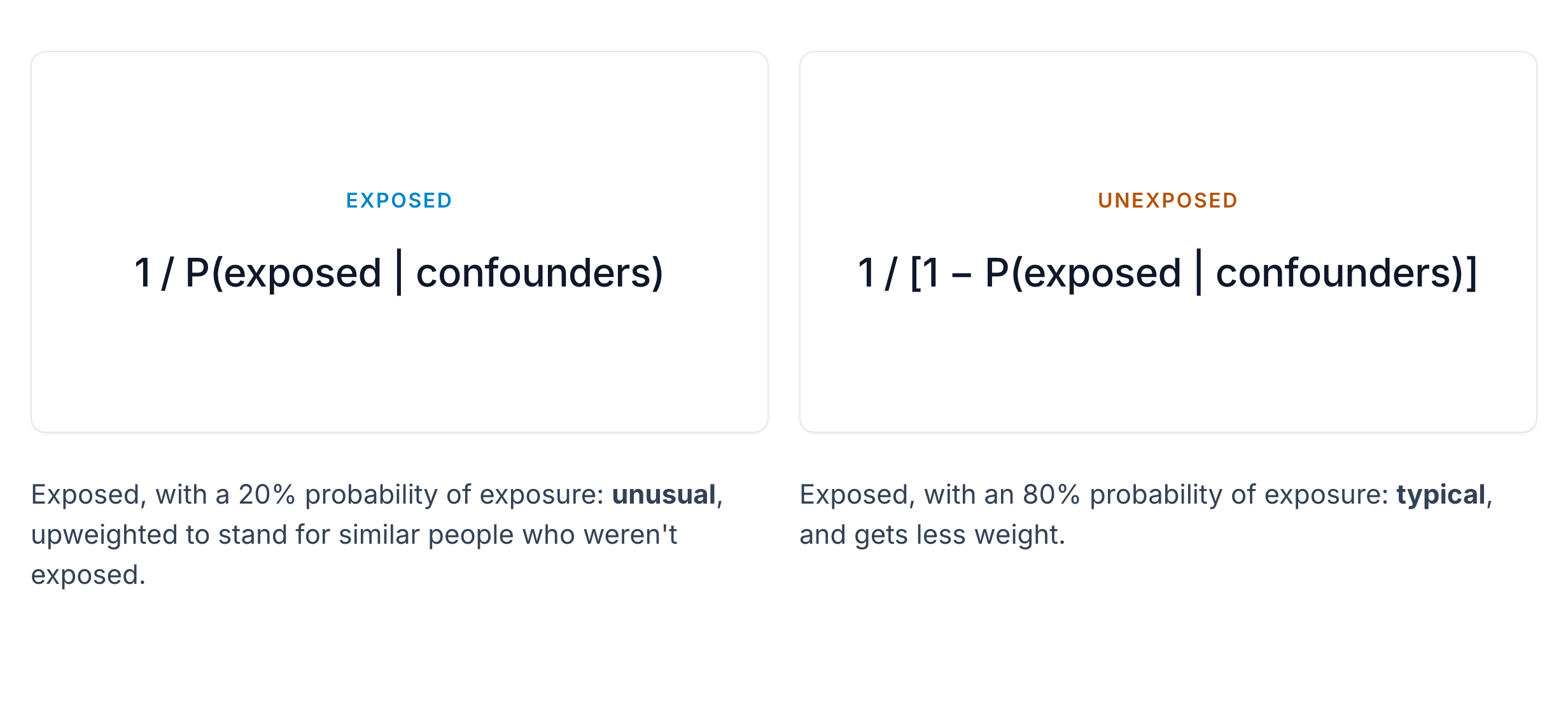
IPTW weights. Each person is weighted by one over the probability of the treatment they actually received.
Slide 13
IPTW
Extreme weights are a warning sign
Uses every observation and estimates population-level effects
Handles time-varying exposures well
Always check the weight distribution
Slide 14
TMLE
TMLE optimizes for the causal parameter we want to estimate
An initial outcome model, which can use machine learning
A propensity score model
A targeting step that updates the outcome model for the causal effect
Slide 15
TMLE
What TMLE offers over regression and propensity score methods
Doubly robust: consistent if either model is correctly specified
Compatible with machine learning, with valid confidence intervals
Efficient among doubly robust estimators
Slide 16
Choosing among methods
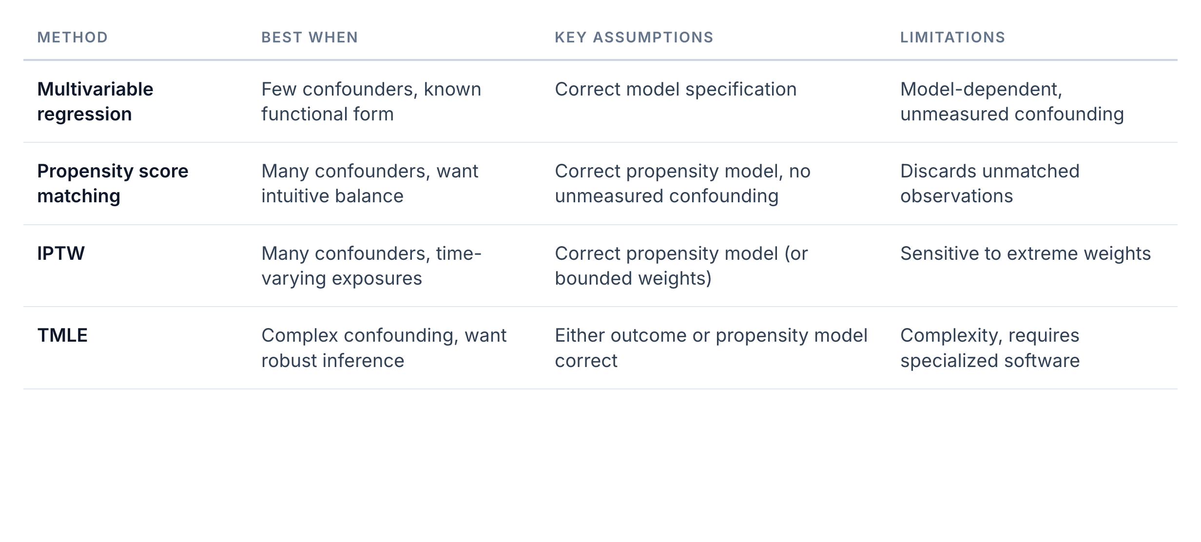
Methods for confounder control, from the chapter. For instrumental variables, regression discontinuity, and difference-in-differences, see the quasi-experimental chapter.
Slide 17
No purely observational method eliminates unmeasured confounding
Combine thoughtful design, appropriate methods, and honest acknowledgment of limitations
How strong would unmeasured confounding need to be to explain away our findings?
Slide 18
In Closing
Statistical adjustment only controls for confounders we measured
Observational studies can provide strong, actionable evidence
The possibility of unmeasured confounding always remains
Controlling confounding in observational data
Slide 1Confounding is the central challenge in all observational research. Each design attempts to address it, but their strategies differ.
Confounder control is the strategy this chapter takes
A confounder is associated with both the exposure and the outcome
It creates a spurious association between them
Slide 2In our session on causal inference, we defined a confounder as a variable associated with both the exposure and the outcome, creating a spurious association between them. We also introduced two strategies for causal inference from non-experimental data. The observational designs in this chapter rely on the first of them: measuring and adjusting for the things that confound the comparison. We can do that at the design phase, at the analysis phase, or both.
Design phase
Design-phase strategies differ by design
Cross-sectional: limited control, beyond sampling for variation in confounders
Case-control: matching cases and controls on potential confounders
Cohort: restriction to a narrow range, or matching unexposed to exposed
Slide 3Cross-sectional studies offer limited confounding control by design. We can stratify the sample to make sure there's variation across potential confounders, but we're measuring everything at once. Case-control studies use matching, making cases and controls similar on potential confounders like age, sex, and geography. Cohort studies can use restriction, only including people within a narrow range of the confounder, say only women aged 40 to 45, or matching unexposed people to exposed ones.
Siddique et al., 2011
Outdoor air pollution and children's respiratory health in Delhi
Did outdoor air pollution affect children's respiratory health?
Children from different backgrounds differ in exposure and in baseline risk
Slide 4A study of air pollution and respiratory health in Delhi shows how confounding control works in practice. Researchers wanted to understand whether outdoor air pollution affected children's respiratory health. But children from different socioeconomic backgrounds have different pollution exposures and different baseline health risks.
Background affects both exposure and outcome
Socioeconomic background as a confounder of pollution and respiratory health, as the chapter describes the Delhi study.
Slide 5Wealthier families might live in less polluted neighborhoods and have better access to healthcare. Poorer families might experience both higher pollution and more crowding, indoor smoke, and nutritional deficits, all of which affect respiratory health. Socioeconomic background sits upstream of both the exposure and the outcome, and unless we deal with it, some of what looks like an effect of pollution is really an effect of background.
Siddique et al., 2011
Matching before the analysis, regression during it
Matched on age, sex, parental education, household income, and neighborhood
Then multivariate logistic regression for further adjustment
Slide 6The study team matched participants on several sociodemographic factors before the analysis even began: age, sex, parental education, household income, and neighborhood characteristics. That design-phase matching meant comparisons between high and low pollution groups wouldn't be confounded by those background variables. But matching alone wasn't enough. In the analysis phase, they used multivariate logistic regression to adjust further, estimating the effect of pollution while holding other factors constant.
Analysis phase
Stratification and multivariable regression ask different questions
Stratification
Present within each stratum?
Transparent, but only a few confounders
Multivariable regression
What is the association after adjustment?
Many confounders at once
Slide 7Stratification means analyzing the exposure-outcome relationship separately within levels of the confounder. It asks whether the pollution-health association is present within each stratum. If it holds across all strata, confounding by that variable is less likely. Multivariable regression asks what the association is after accounting for all measured confounders simultaneously. Both approaches aim to isolate pollution's effect from other influences.
Assimon et al., 2021
A propensity score models the probability of exposure
Each person's probability of being exposed, given their characteristics
Then match, stratify, or weight on that single score
Slide 8Propensity score methods are a more sophisticated approach. First, we build a statistical model predicting exposure, not outcome, from all the measured confounders. That gives each person a propensity score, their probability of being exposed given their characteristics. Then we use those scores to make exposed and unexposed groups comparable. We might match people with similar scores, stratify by score quintiles, or weight each person by the inverse of their propensity to be in the group they're in.
Assimon et al., 2021
Why condense many confounders into one score
Regression with many confounders can become unstable in modest samples
One number makes matching and balance checks more straightforward
Slide 9Why go through all this? When there are many potential confounders, traditional regression can become unstable, especially with modest sample sizes. Propensity scores condense all that information into a single number, which makes matching and checking balance more straightforward. They're particularly useful in observational studies trying to mimic randomized trials.
Target trial emulation
Approximating the conditions of a randomized experiment
No statistical method can fully substitute for randomization
Unmeasured confounding remains a fundamental limitation
Slide 10As observational research has matured, so have methods for extracting causal estimates from non-randomized data. These approaches aim to make observational studies approximate the conditions of a randomized experiment, what methodologists call target trial emulation. No statistical method can fully substitute for randomization, because unmeasured confounding remains a fundamental limitation, but these techniques are our best tools when experiments aren't possible.
IPTW
Inverse probability of treatment weighting creates a pseudo-population
Exposure becomes independent of measured confounders
The sample is reweighted to mimic random assignment
Slide 11Inverse probability of treatment weighting, or IPTW, takes the propensity score further. Instead of matching or stratifying, it creates a pseudo-population in which exposure is independent of the measured confounders, reweighting the sample to mimic random assignment.
Weighted by the inverse probability of the treatment received
IPTW weights. Each person is weighted by one over the probability of the treatment they actually received.
Slide 12Here's the intuition. If a person had a low probability of being exposed, say 20%, but was exposed, they're unusual among exposed people. We upweight them, so they represent not just themselves but all the similar people who weren't exposed. Someone with an 80% probability who was exposed is typical, and gets less weight. Each person's weight is one over the probability of the treatment they actually received.
IPTW
Extreme weights are a warning sign
Uses every observation and estimates population-level effects
Handles time-varying exposures well
Always check the weight distribution
Slide 13IPTW uses every observation, handles time-varying exposures well, and estimates population-level effects. The trade-off is sensitivity to extreme weights. If some people have very low propensity scores but were exposed, their weights become enormous and the estimates become unstable. So we always check the weight distribution. A handful of people with weights of 50 or 100 are warning signs. In global health, IPTW is increasingly used with clinical cohorts, for example to compare mortality between patients started on different first-line ART regimens.
TMLE
TMLE optimizes for the causal parameter we want to estimate
An initial outcome model, which can use machine learning
A propensity score model
A targeting step that updates the outcome model for the causal effect
Slide 14Targeted maximum likelihood estimation, or TMLE, combines machine learning with causal inference. The key insight is that standard regression minimizes prediction error across the whole outcome distribution, but we only care about a specific causal estimand, like the average treatment effect. TMLE is targeted because it optimizes for that parameter. It works in three stages: an initial outcome model, which can use machine learning, a propensity score model, and a targeting step that updates the outcome model using information from the propensity score.
TMLE
What TMLE offers over regression and propensity score methods
Doubly robust: consistent if either model is correctly specified
Compatible with machine learning, with valid confidence intervals
Efficient among doubly robust estimators
Slide 15TMLE has properties simpler methods lack. First, it's doubly robust. Estimates remain consistent if either the outcome model or the propensity model is correctly specified, where regression needs the outcome model to be right and IPTW needs the propensity model to be right. Second, it's compatible with machine learning, so it handles situations where we don't know the functional form, while still providing valid confidence intervals. Third, among doubly robust estimators, it's efficient. The downside is complexity: it requires specialized software and an understanding of causal inference concepts.
Choosing among methods
Methods for confounder control, from the chapter. For instrumental variables, regression discontinuity, and difference-in-differences, see the quasi-experimental chapter.
Slide 16Choosing among these methods depends on how many confounders there are, whether exposures vary over time, and what we're willing to assume. Regression works with few confounders and a known functional form. Propensity score matching gives intuitive balance but discards unmatched observations. IPTW handles many confounders and time-varying exposures, but it's sensitive to extreme weights. And TMLE offers robust inference at the cost of complexity.
No purely observational method eliminates unmeasured confounding
Combine thoughtful design, appropriate methods, and honest acknowledgment of limitations
How strong would unmeasured confounding need to be to explain away our findings?
Slide 17The honest answer is that no purely observational method eliminates unmeasured confounding. The best approach combines thoughtful study design, measuring the important confounders, with appropriate methods and honest acknowledgment of limitations. Sensitivity analyses help quantify robustness by asking: how strong would unmeasured confounding need to be to explain away our findings?
In Closing
Statistical adjustment only controls for confounders we measured
Observational studies can provide strong, actionable evidence
The possibility of unmeasured confounding always remains
Slide 18Statistical adjustment only controls for confounders we've measured. If there's an unmeasured variable associated with both exposure and outcome, no amount of fancy statistics will save us. That's why observational studies, no matter how well designed, can never prove causation the way randomized trials can. They can provide strong evidence, compelling evidence, actionable evidence. But there's always the possibility of unmeasured confounding.