Chapter 7 · Video 4
Good paths and bad paths
Print layout
Slide 1


Good paths and bad paths
Slide 2
Trace every path from the cause to the outcome
Move along each path until you reach another variable or the outcome
The direction of the arrows does not matter for tracing
No loops — never trace back to a variable you have already visited
Slide 3
Five paths from road traveled to happiness
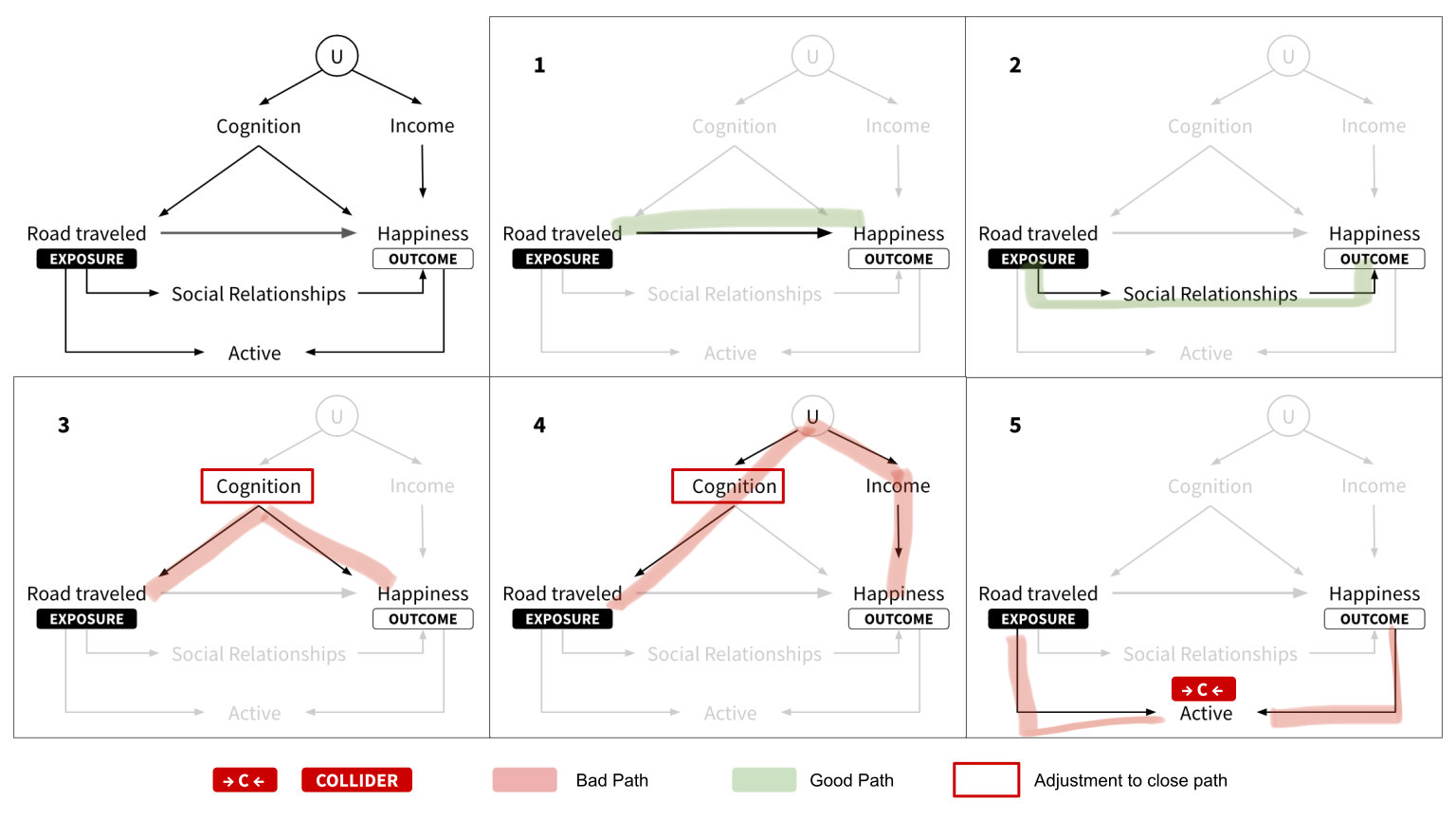
Good and bad paths in our example DAG. Reproduced from Chapter 7.
Slide 4
Check your work, or skip the tracing entirely
Build the DAG visually in your browser at DAGitty.net
Copy and paste the model code into R
The `paths()` function returns the same five paths
Slide 5
Huntington-Klein, 2021
Good paths identify the question; bad paths are the alternatives
Good paths often start with an arrow exiting the proposed cause
Bad paths have arrows entering the proposed cause
Bad paths are what we need to close
Slide 6
Paths 1 and 2 flow forward from the cause
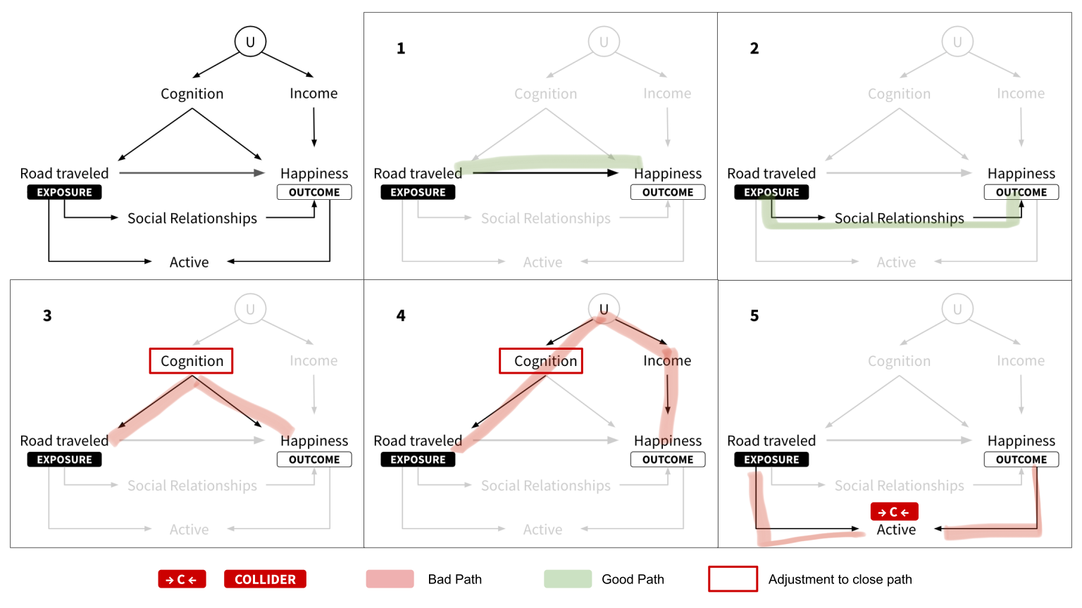
Panels 1 and 2 are the good paths: they start at road traveled and flow forward to happiness. Reproduced from Chapter 7.
Slide 7
Paths 3, 4, and 5 are backdoor paths
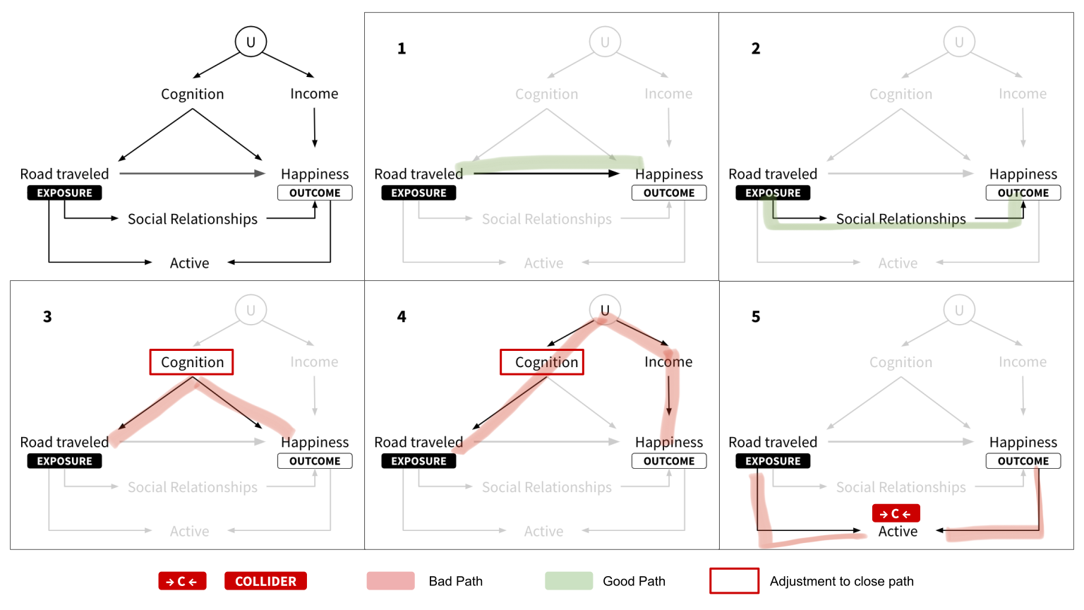
Panels 3, 4, and 5 are backdoor paths. Open backdoor paths bias the causal effect we want to estimate. Reproduced from Chapter 7.
Slide 8
A minimum sufficient set, not every possible confounder
Condition on the confounders through techniques like regression
You need enough to close all backdoor paths, and no more
`dagitty::adjustmentSets()` will find them for you
Slide 9
Adjusting for cognition closes paths 3 and 4
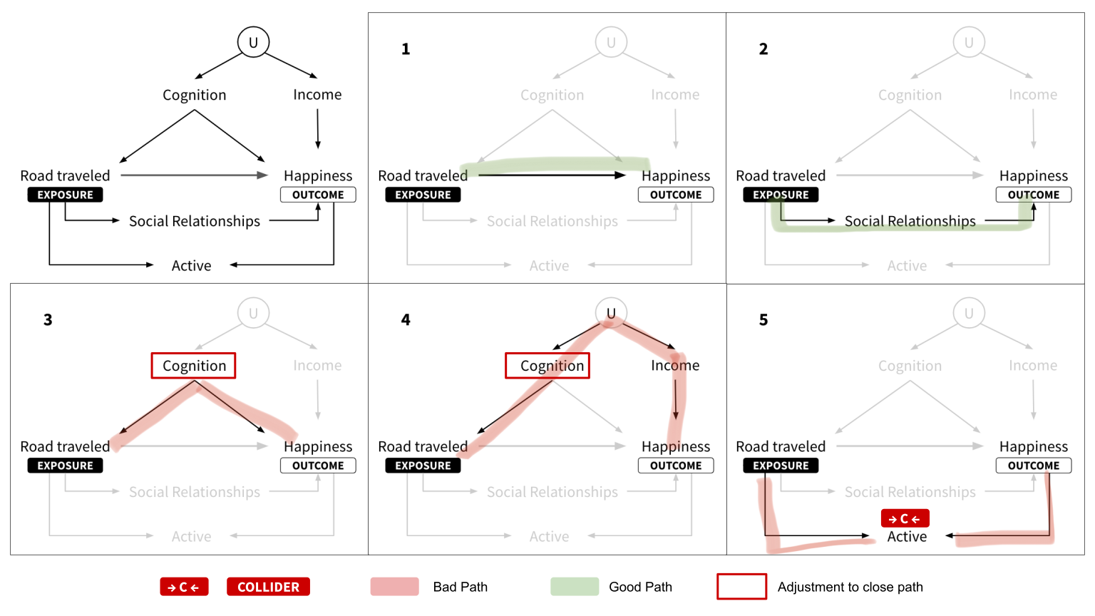
Cognition is boxed in panels 3 and 4: one adjustment closes both open backdoor paths. Reproduced from Chapter 7.
Slide 10
Path 5 is closed by default, because active is a collider
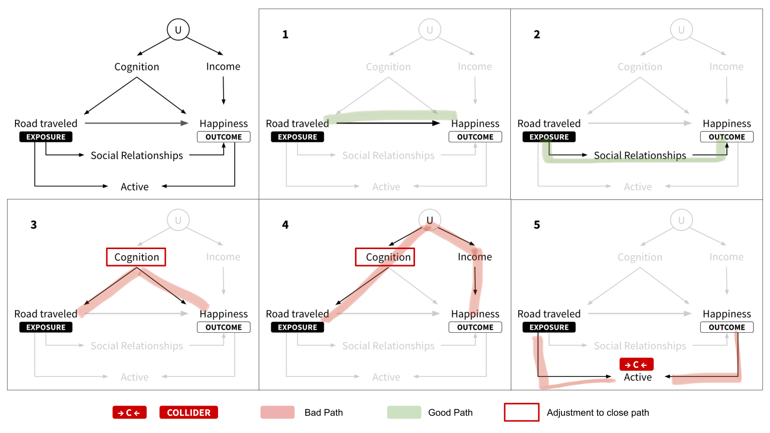
Panel 5. Two arrows enter active, so the path is closed until you condition on it. Reproduced from Chapter 7.
Slide 11
Westreich, 2013 · McElreath, 2020
There is such a thing as a bad covariate
Sometimes less is more when it comes to statistical models
Need a variable that isn't in your dataset? You might be out of luck
The longer answer involves creativity, some assumptions, and math
Slide 12
The causal effect is identified
If this DAG is correct and complete
Adjusting for cognition d-separates road traveled from all other nodes
d-separated means direction separated
Slide 13
"I've read plenty of papers that adjust for confounding"
None of them drew a DAG
Age, sex, education, wealth — controlled for, with no diagram
Are we doing something different here? Yes and no.
Slide 14
Yes and no
Yes
Explicit about causal assumptions
Forces you to say why you adjust
A tool for clarity and honesty
No
The statistical machinery is the same
"Controlling for" is that adjustment
The causal model was in their heads
Slide 15
In Closing
The difference is transparency
Without a DAG, assumptions often go unstated, but they are still there
Every choice about what to adjust for reflects a belief about structure
DAGs make those beliefs visible to you, to your readers, to your critics
Good paths and bad paths
Slide 1Once you've drawn your DAG, the next step is to list all of the paths from the proposed cause to the outcome of interest. In this example, it means tracing all of the paths that go from road traveled to happiness.
Trace every path from the cause to the outcome
Move along each path until you reach another variable or the outcome
The direction of the arrows does not matter for tracing
No loops — never trace back to a variable you have already visited
Slide 2Start with road traveled and move your finger along each path until you get to another variable or to the outcome, happiness. When you encounter variables with arrows coming in or out, trace each path to the outcome. The direction of the arrows does not matter for tracing. Just don't trace back to variables you've already visited. In other words, no loops.
Five paths from road traveled to happiness
Good and bad paths in our example DAG. Reproduced from Chapter 7.
Slide 3In our example DAG there are five paths. Path one: road traveled leads directly to happiness. Path two: road traveled leads to social relationships, which leads to happiness. Path three: cognition points to both road traveled and happiness. Path four: background points to cognition, and background also points to income, which points to happiness. And path five: road traveled points to active, and happiness points to active as well.
Check your work, or skip the tracing entirely
Build the DAG visually in your browser at DAGitty.net
Copy and paste the model code into R
The `paths()` function returns the same five paths
Slide 4You can check your work, or skip the manual tracing process entirely, by creating and analyzing your DAG in R. While you can manually enter your graph into R, a shortcut is to create your DAG visually in your browser at DAGitty dot net, and copy and paste the model code into R. The paths function returns the same five paths we traced by hand.
Huntington-Klein, 2021
Good paths identify the question; bad paths are the alternatives
Good paths often start with an arrow exiting the proposed cause
Bad paths have arrows entering the proposed cause
Bad paths are what we need to close
Slide 5Next we need to determine which paths are good and which are bad. Good paths identify our research question. Bad paths are the alternate explanations for the causal effect that we need to close. In our example DAG, as in many DAGs, good paths often start with an arrow exiting the proposed cause, and bad paths have arrows entering the proposed cause.
Paths 1 and 2 flow forward from the cause
Panels 1 and 2 are the good paths: they start at road traveled and flow forward to happiness. Reproduced from Chapter 7.
Slide 6Here the five paths are labeled good or bad. Notice that paths one and two, the good paths, start with road traveled and flow forward to happiness. Those are the paths that carry the causal effect we're trying to estimate.
Paths 3, 4, and 5 are backdoor paths
Panels 3, 4, and 5 are backdoor paths. Open backdoor paths bias the causal effect we want to estimate. Reproduced from Chapter 7.
Slide 7The rest are backdoor paths that we need to close. Paths three and four have an arrow entering road traveled. Path five is a backdoor path as well, and it behaves differently, which we'll come to in a moment. Open backdoor paths bias the causal effect we want to estimate, so we need to close them.
A minimum sufficient set, not every possible confounder
Condition on the confounders through techniques like regression
You need enough to close all backdoor paths, and no more
`dagitty::adjustmentSets()` will find them for you
Slide 8We can do this by conditioning on variables that confound the causal effect of interest, through techniques like regression. The neat thing is that we do not necessarily need to control for every possible confounder, just a minimum set sufficient to close all backdoor paths. Both DAGitty and the adjustment sets function in R will tell us which variables make up minimally sufficient adjustment sets.
Adjusting for cognition closes paths 3 and 4
Cognition is boxed in panels 3 and 4: one adjustment closes both open backdoor paths. Reproduced from Chapter 7.
Slide 9In this figure, you can see that adjusting for cognition in paths three and four is sufficient to close the open backdoor paths. Cognition is boxed in both of those panels, because one adjustment closes both.
Path 5 is closed by default, because active is a collider
Panel 5. Two arrows enter active, so the path is closed until you condition on it. Reproduced from Chapter 7.
Slide 10Path five is also a backdoor path, but it's closed by default, because active is a collider. Look at the two incoming arrows. If we condition on active, let's say by including it as a covariate in our regression, we will inadvertently open this path and introduce bias.
Westreich, 2013 · McElreath, 2020
There is such a thing as a bad covariate
Sometimes less is more when it comes to statistical models
Need a variable that isn't in your dataset? You might be out of luck
The longer answer involves creativity, some assumptions, and math
Slide 11There is such a thing as a bad covariate, and sometimes less is more when it comes to statistical models. And what if you need to adjust for a variable that's not in your dataset? The short answer is that you might be out of luck. The longer answer is more optimistic, but it probably involves creativity, some assumptions, and math.
The causal effect is identified
If this DAG is correct and complete
Adjusting for cognition d-separates road traveled from all other nodes
d-separated means direction separated
Slide 12If this DAG is correct and complete, adjusting for cognition on the backdoor path makes the relationship between road traveled and happiness d-separated, or direction separated, from all other nodes. In other words, the causal effect is said to be identified.
"I've read plenty of papers that adjust for confounding"
None of them drew a DAG
Age, sex, education, wealth — controlled for, with no diagram
Are we doing something different here? Yes and no.
Slide 13Now, you may have read lots of papers that adjust for confounding, and none of them used a DAG. You're right, and this is worth pausing on. If you've been reading the global health literature, you've seen countless papers that control for age, sex, education, wealth, and other variables without ever drawing a diagram. Are we doing something different here?
Yes and no
Yes
Explicit about causal assumptions
Forces you to say why you adjust
A tool for clarity and honesty
No
The statistical machinery is the same
"Controlling for" is that adjustment
The causal model was in their heads
Slide 14Yes and no. Yes, in the sense that we're being explicit about our causal assumptions. The DAG forces us to think carefully about why we're adjusting for certain variables, and to communicate those reasons transparently. It's a tool for clarity and honesty. And no, in the sense that the underlying statistical machinery is the same. When a paper controls for confounders in a regression model, it's doing the same kind of adjustment we just described. It's simply not showing its work. The authors still had to make decisions about which variables to include and exclude, which means they had a causal model in their heads, whether or not they drew it.
In Closing
The difference is transparency
Without a DAG, assumptions often go unstated, but they are still there
Every choice about what to adjust for reflects a belief about structure
DAGs make those beliefs visible to you, to your readers, to your critics
Slide 15The difference is transparency. Without a DAG, assumptions often go unstated, but they're still there. Every choice about what to adjust for reflects beliefs about causal structure. DAGs just make those beliefs visible, to you, to your readers, and to your critics.