Chapter 11 · Video 4
Interrupted time series and the kidney transplant wait-time policy
Print layout
Slide 1


Interrupted time series
Slide 2
When there is no untreated group to compare against
A national policy that affects every district at once
A hospital system that changes its protocol everywhere
The unit's own past becomes the counterfactual
Slide 3
Interrupted time series
A change in level, a change in slope, or both?
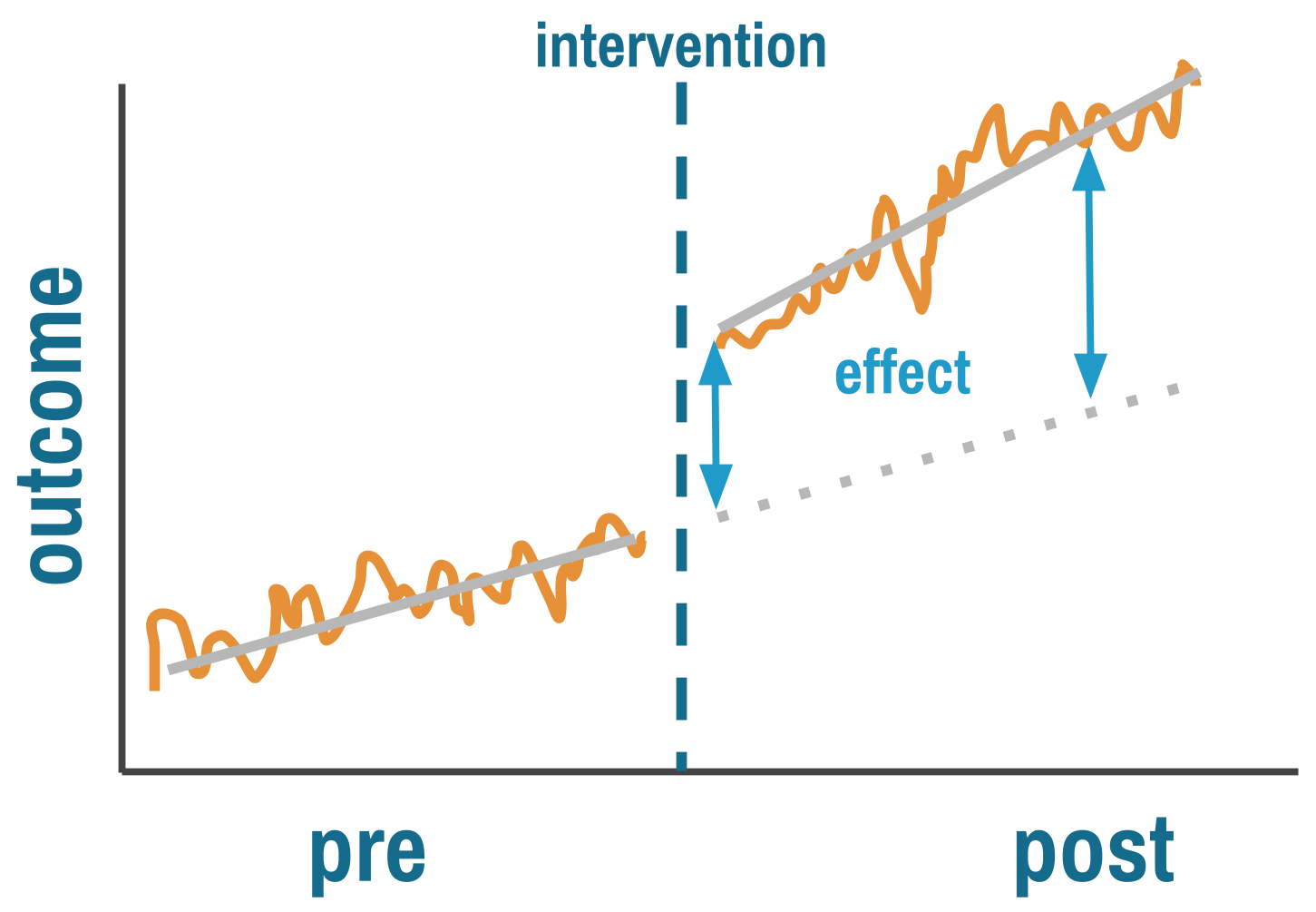
Interrupted time series design. Reproduced from Chapter 11.
Slide 4
Segmented regression
Yt = β0 + β1·time + β2·intervention + β3·time after intervention + εt
β2 captures the immediate level change
β3 captures the change in slope after the intervention
Slide 5
Reading an interrupted time series plot
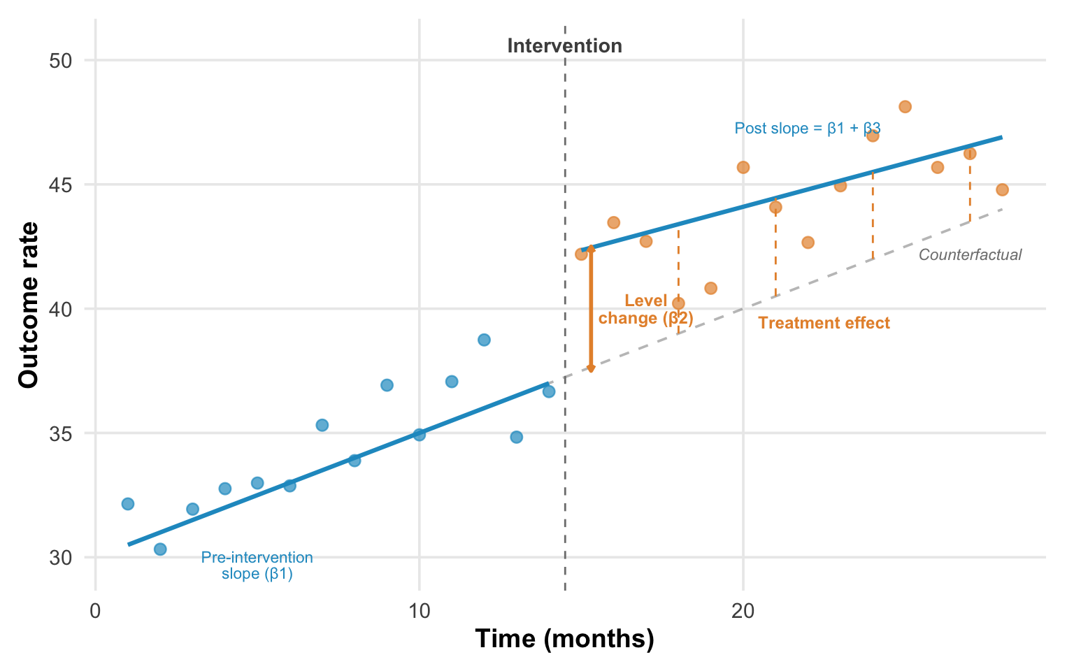
The pre-intervention slope is projected forward as the counterfactual (dashed gray). The treatment effect at any point is the gap between the observed trend and the counterfactual. Reproduced from Chapter 11.
Slide 6
What does a credible break in the trend look like?
A stable pre-intervention trend, with points close to the fitted line
A clear jump or drop at the intervention
A new level or trend sustained across many observations
Slide 7
What does confounding look like on the same plot?
A pre-intervention trend already moving toward the apparent effect
Erratic post-intervention points
Effects appearing before the intervention line
Slide 8
Main threat
Concurrent events
Anything else that changed at the same time is an alternative explanation
A hand hygiene campaign that launched in March 2020
Slide 9
Autocorrelation, seasonality and regression to the mean
Correlated observations make standard errors too small
A seasonal pattern can be mistaken for an intervention effect
Interventions often follow unusual values, like an outbreak
Slide 10
How many time points does the design need?
A conventional minimum of 8 before and 8 after
12 or more on each side is far better
With fewer, it offers little over a pre-post comparison
Slide 11
Kidney transplantation
The race coefficient in kidney function equations
Systematically overstated kidney health in Black patients
Later referral, later listing, shorter effective wait times
2021: a task force recommended removing it
January 2023: retroactive wait time modifications mandated
Slide 12
Khazanchi et al., 2026
Monthly transplant rates before and after January 2023
Outcome: transplants per 1,000 waitlisted candidates, by month
Rates were already rising slowly before the policy
A three-month washout for gradual implementation
Slide 13
Khazanchi et al., 2026
The change in transplant rates for Black candidates
Immediate level change
+5.3 per 1,000 listings
95% CI 3.5 to 7.0
Mostly deceased donor transplants
Slope after the policy
−0.10 per month
The initial jump faded
Slide 14
In Closing
Who the policy reached
Less than one-third of eligible Black candidates received modifications
Beneficiaries were already integrated into the healthcare system
Patients never listed were out of reach
Interrupted time series
Slide 1Difference-in-differences relies on a comparison group to construct the counterfactual. But what if we don't have one?
When there is no untreated group to compare against
A national policy that affects every district at once
A hospital system that changes its protocol everywhere
The unit's own past becomes the counterfactual
Slide 2Think of a national policy that affects every district simultaneously, a hospital system that changes its protocol everywhere at once, or a country-wide ban on a class of antibiotics. There's no untreated group to compare against. Interrupted time series designs handle this by replacing the comparison group with the unit's own past. If we have enough data points before and after the intervention, we can model the pre-intervention trend and ask whether the intervention interrupted it. Some researchers call this an event study design, particularly when the focus is on estimating dynamic effects around a discrete event.
Interrupted time series
A change in level, a change in slope, or both?
Interrupted time series design. Reproduced from Chapter 11.
Slide 3An interrupted time series answers two questions at once. Did the intervention cause an immediate level change, a sudden jump or drop at the moment it was implemented? And did it cause a trend change, a shift in the slope of the outcome over time? The pre-intervention trend, extrapolated forward, represents what would have happened without the intervention.
Segmented regression
Yt = β0 + β1·time + β2·intervention + β3·time after intervention + εt
β2 captures the immediate level change
β3 captures the change in slope after the intervention
Slide 4The design is typically implemented using segmented regression. One coefficient captures the immediate level change, and another captures the change in slope after the intervention. The key assumption is that the pre-intervention trend would have continued unchanged, and that nothing else happened at the same time as the intervention that could explain the break.
Reading an interrupted time series plot
The pre-intervention slope is projected forward as the counterfactual (dashed gray). The treatment effect at any point is the gap between the observed trend and the counterfactual. Reproduced from Chapter 11.
Slide 5The classic plot has time on the x-axis, outcome on the y-axis, and a vertical line marking the intervention. At the intervention, we look for two things. A level change: does the outcome jump or drop immediately? And a slope change: does the trajectory's angle shift? The dashed gray line shows the counterfactual: where the outcome would have gone if the pre-intervention trend had simply continued. The treatment effect at any point after the intervention is the vertical gap between the counterfactual and the observed post-intervention trend.
What does a credible break in the trend look like?
A stable pre-intervention trend, with points close to the fitted line
A clear jump or drop at the intervention
A new level or trend sustained across many observations
Slide 6A credible effect looks like a stable pre-intervention trend, with points clustered tightly around the fitted line, then a clear discontinuity, followed by a sustained new level or trend confirmed by multiple post-intervention observations. The key word is sustained. A single outlier after the intervention doesn't mean much, but a consistent shift across many subsequent data points does.
What does confounding look like on the same plot?
A pre-intervention trend already moving toward the apparent effect
Erratic post-intervention points
Effects appearing before the intervention line
Slide 7What does confounding look like? A pre-intervention trend already moving in the direction of the apparent effect, where we're seeing continuation and not interruption. Erratic post-intervention points, suggesting other factors are varying at the same time. Or effects appearing before the intervention line, suggesting the timing in the model doesn't match the actual implementation. Each of these patterns is a reason to question whether the break in the trend is real.
Main threat
Concurrent events
Anything else that changed at the same time is an alternative explanation
A hand hygiene campaign that launched in March 2020
Slide 8The central threat is concurrent events. Because the counterfactual is the projected pre-intervention trend, anything else that changed at the same time as the intervention becomes an alternative explanation. Imagine evaluating a hand hygiene campaign that launched in March 2020. Any improvement we observe could be the campaign or the pandemic response that started simultaneously, and the design has no way to separate the two without additional information.
Autocorrelation, seasonality and regression to the mean
Correlated observations make standard errors too small
A seasonal pattern can be mistaken for an intervention effect
Interventions often follow unusual values, like an outbreak
Slide 9This vulnerability is compounded by several technical challenges. Observations close in time are correlated, which makes standard errors too small if we don't account for it. Outcomes that fluctuate with the seasons require explicit seasonal adjustment, or the model will confuse a seasonal pattern with an intervention effect. And interventions often follow unusual values, like safety protocols implemented after an outbreak, which means regression to the mean can masquerade as a treatment effect. The outbreak was extreme, and things would have improved anyway.
How many time points does the design need?
A conventional minimum of 8 before and 8 after
12 or more on each side is far better
With fewer, it offers little over a pre-post comparison
Slide 10Finally, the design is data-hungry. The conventional minimum is 8 time points before and after, though 12 or more on each side is far better. With fewer, we're fitting a line to noise, and the design offers little advantage over a simple pre-post comparison.
Kidney transplantation
The race coefficient in kidney function equations
Systematically overstated kidney health in Black patients
Later referral, later listing, shorter effective wait times
2021: a task force recommended removing it
January 2023: retroactive wait time modifications mandated
Slide 11For decades, the equations used to estimate kidney function included a race coefficient that systematically overstated kidney health in Black patients. Black patients appeared healthier than they were, leading to later referrals, later listing for transplant, and shorter effective wait times once listed. In 2021, a task force recommended removing the race coefficient. In January 2023, the Organ Procurement and Transplantation Network went further and mandated retroactive wait time modifications for Black candidates whose listing had been delayed by the old equations. More than 21,000 candidates received modifications, gaining a median of 1.7 additional years of wait time.
Khazanchi et al., 2026
Monthly transplant rates before and after January 2023
Outcome: transplants per 1,000 waitlisted candidates, by month
Rates were already rising slowly before the policy
A three-month washout for gradual implementation
Slide 12Researchers used an interrupted time series to evaluate whether this policy change actually increased kidney transplants for Black candidates. The outcome is the monthly transplant rate per 1,000 waitlisted candidates. The pre-intervention period establishes the trend: transplant rates were already rising slowly for both Black and non-Black candidates before the policy. The intervention has a known date, and the authors excluded a three-month washout period to account for gradual implementation.
Khazanchi et al., 2026
The change in transplant rates for Black candidates
Immediate level change
+5.3 per 1,000 listings
95% CI 3.5 to 7.0
Mostly deceased donor transplants
Slope after the policy
−0.10 per month
The initial jump faded
Slide 13Black candidates experienced an immediate level change of 5.3 transplants per 1,000 listings, with a 95% confidence interval from 3.5 to 7.0, driven almost entirely by deceased donor transplants. The post-intervention slope then declined slightly, suggesting the initial jump faded as the backlog of modified candidates was absorbed.
In Closing
Who the policy reached
Less than one-third of eligible Black candidates received modifications
Beneficiaries were already integrated into the healthcare system
Patients never listed were out of reach
Slide 14The study also illustrates what the design can't tell us. Less than one-third of eligible Black candidates actually received wait time modifications. The beneficiaries were disproportionately patients who had a nephrologist, who had been referred, who were already listed. The policy corrected algorithmic harm for people the system could see, but it couldn't reach patients who never made it to the transplant list in the first place. The design can measure the effect of a policy on those it touched, and it can't measure what the policy missed.