Chapter 6 · Video 3
Retaining or rejecting the null hypothesis
Print layout
Slide 1


Retaining or rejecting the null hypothesis
Slide 2
Step 3
Set the goal posts before you conduct the study
If the result crosses the threshold, it is deemed statistically significant
If it falls short, the null hypothesis of no difference is retained
That threshold is the alpha level
Slide 3
Alpha is how willing you are to be wrong in the long run
It applies to rejecting the null hypothesis
Traditionally, scientists set alpha to be no greater than 5%
Lakens and colleagues argue the optimal alpha is sometimes lower and sometimes higher
Slide 4
5% of the distribution falls outside the lines
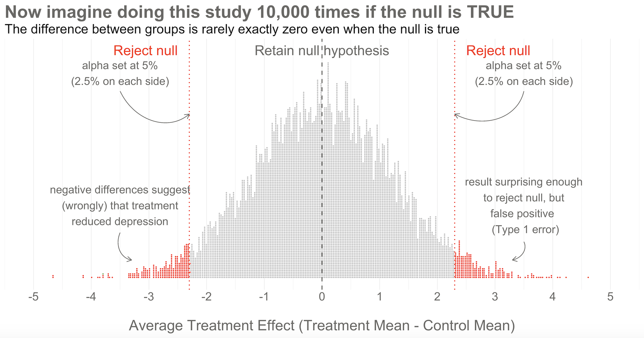
The goal posts, drawn as dotted red lines on the 10,000 simulated studies with no true effect. 2.5% of results sit in each tail, because this is a two-tailed test. Reproduced from Chapter 6.
Slide 5
Step 4
With the goal posts set, the decision is automatic
Your study result falls inside the goal posts, or outside them
You must either retain or reject the null hypothesis
Statistical inference happens on the null
Slide 6
Study #7,501 came back with a difference of -3.8. Retain, or reject?
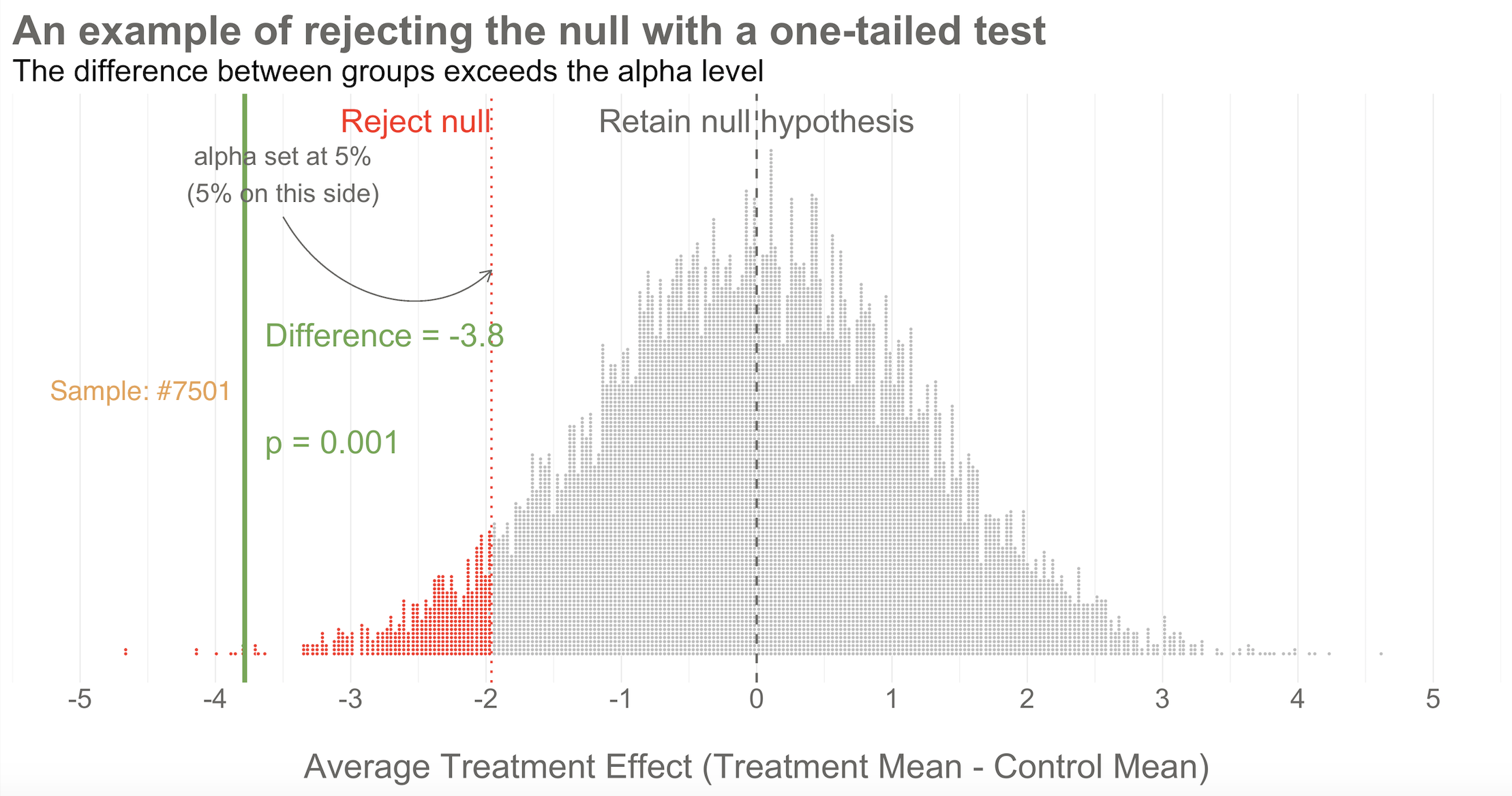
10,000 simulated results when there's no effect. Result of study #7,501 falls outside of the goal post, so the null hypothesis is rejected. Reproduced from Chapter 6.
Slide 7
Reject — and the result is labeled statistically significant
A difference of -3.8 falls outside the alpha level you set at 5%
It sits at the first percentile of our simulated collective
An extreme result relative to what we expected if the null is true
Slide 8
The p-value is a conditional probability
The probability of observing a result as big or bigger than -3.8
IF the null hypothesis is true
Here, that probability is 1%
Slide 9
The p-value might not mean what you want it to mean
P(D|H)
The probability of observing the data
If the null hypothesis is true
What a p-value gives you
P(H|D)
The probability the null is true
Given the data you observed
Which we never get to know
Slide 10
Type I error
We rejected a null hypothesis that was true by construction
We called the result statistically significant. It is a false positive
In the long run we will only make this mistake 5% of the time
We have no way of knowing whether THIS experiment is one of those times
Slide 11
Type II error
The other mistake is a false negative
The treatment really does have an effect
But we fail to reject the null
False negatives and power come later, in the sample size chapter
Slide 12
An imaginary population, and one sample of 332 drawn from it
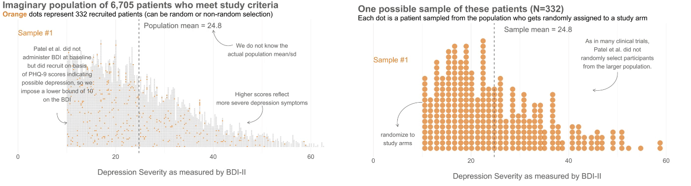
One of 20 simulated studies, each drawing its own sample from 6,705 people who meet the study criteria. Frames from the animated figure in Chapter 6.
Slide 13
Each sample is split at random: half to treatment, half to control
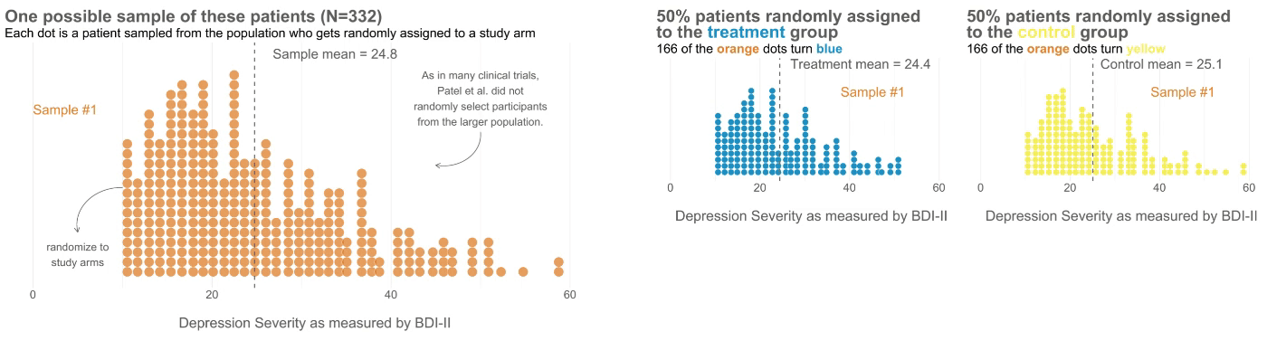
The 332 sampled patients are randomly assigned, 166 to each arm, and each of the 20 studies does this with its own sample. Frames from the animated figure in Chapter 6.
Slide 14
The treatment does nothing, so both arms improve by the same 5 points

Depression falls by 5 points in both groups, yet the two arm means still differ a little by chance. Frames from the animated figure in Chapter 6.
Slide 15
Twenty studies where the treatment does nothing. One rejects the null.
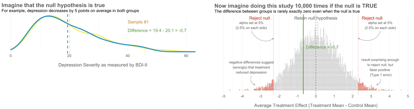
Each study's difference is a green line on 10,000 simulated results. Study #7,501, at -3.8, is the only one of the 20 past the goal post. Frames from the animated figure in Chapter 6.
Slide 16

Patel et al., 2017
What the trial actually found
The program reduced depression severity by an average of 7.57 points
95% confidence interval: -10.27 to -4.86
A difference of that size is off the chart of the null distribution
Slide 17
In Closing
You would expect a difference that big less than 0.01% of the time
The 95% interval excludes the null effect of 0, so the p-value is under 5%
The reported p-value was less than 0.0001
That is the condition talking: if the null hypothesis is true
Retaining or rejecting the null hypothesis
Slide 1In the last video we built an imaginary world of 10,000 studies in which the treatment did nothing. This video sets the goal posts on that curve, makes the decision the Frequentist approach tells us to make, and then shows you what it looks like when that decision is wrong.
Step 3
Set the goal posts before you conduct the study
If the result crosses the threshold, it is deemed statistically significant
If it falls short, the null hypothesis of no difference is retained
That threshold is the alpha level
Slide 2A skeptical student might say, "I get that a study result does not have to be exactly zero for the null to be true. But how different from zero must a result be for Frequentists to reject the null hypothesis that the treatment had no effect?" Good question. In the Frequentist approach, you decide if the data are extreme relative to what is plausible under the null by setting some goal posts before you conduct the study. If the result crosses the threshold, it's automatically deemed statistically significant and the null hypothesis is rejected. If it falls short, the null hypothesis of no difference is retained. This threshold is known as the alpha level.
Alpha is how willing you are to be wrong in the long run
It applies to rejecting the null hypothesis
Traditionally, scientists set alpha to be no greater than 5%
Lakens and colleagues argue the optimal alpha is sometimes lower and sometimes higher
Slide 3For Frequentists, alpha represents how willing they are to be wrong in the long run when it comes to rejecting the null hypothesis. Traditionally, scientists set alpha to be no greater than 5%. That convention has been questioned. One argument is that the optimal alpha level will sometimes be lower and sometimes be higher than the current convention of 0.05, which they describe as arbitrary. Think before you experiment and justify your alpha.
5% of the distribution falls outside the lines
The goal posts, drawn as dotted red lines on the 10,000 simulated studies with no true effect. 2.5% of results sit in each tail, because this is a two-tailed test. Reproduced from Chapter 6.
Slide 4Returning to our simulated results, you can see that I drew the goal posts as dotted red lines. They are positioned so that 5% of the distribution of study results falls outside of the lines, 2.5% in each tail. This is a two-tailed test, meaning that we'd look for a result in either direction. The treatment group gets better, on the left, a negative difference. Or worse, on the right. You can also draw a single goal post that contains the full alpha level. That's appropriate when you have a directional alternative hypothesis.
Step 4
With the goal posts set, the decision is automatic
Your study result falls inside the goal posts, or outside them
You must either retain or reject the null hypothesis
Statistical inference happens on the null
Slide 5Step 4 is to make a decision about the null. With the goal posts set, the decision is automatic. Your actual study result either falls inside or outside the goal posts, and you must either retain or reject the null hypothesis. I'll say it again: statistical inference happens on the null.
Study #7,501 came back with a difference of -3.8. Retain, or reject?
10,000 simulated results when there's no effect. Result of study #7,501 falls outside of the goal post, so the null hypothesis is rejected. Reproduced from Chapter 6.
Slide 6Going back to our example, imagine that you actually conducted study number 7,501 of 10,000. When you collected endline data, you found a mean difference between the two arms of negative 3.8. What's your decision with respect to the null? Do you retain, or reject?
Reject — and the result is labeled statistically significant
A difference of -3.8 falls outside the alpha level you set at 5%
It sits at the first percentile of our simulated collective
An extreme result relative to what we expected if the null is true
Slide 7Reject. A difference of negative 3.8 falls outside of the alpha level you set at 5%. Therefore, you automatically reject the null hypothesis and label the result statistically significant. But there's something else we know about this result, the raw effect size of negative 3.8. It falls at the first percentile of our simulated collective. It's an extreme result relative to what we expected if the null is true. We'd say it has a p-value of 1%.
The p-value is a conditional probability
The probability of observing a result as big or bigger than -3.8
IF the null hypothesis is true
Here, that probability is 1%
Slide 8The p-value is a conditional probability. It's the probability of observing a result as big or bigger than our study result, negative 3.8, and here's the conditional part, if the null hypothesis is true.
The p-value might not mean what you want it to mean
P(D|H)
The probability of observing the data
If the null hypothesis is true
What a p-value gives you
P(H|D)
The probability the null is true
Given the data you observed
Which we never get to know
Slide 9I can hear you muttering to yourself. I think you said, "Why does he keep saying if the null hypothesis is true, like some lawyer who loves fine print?" I do love fine print, but it's important to say this again. When it comes to inference, we never know the truth. We do not know if the null hypothesis is actually true or false. That's why the p-value is a conditional probability. A p-value is the probability of observing the data if the null hypothesis is true, not the probability that the null hypothesis is true given the data. Let that sink in. The p-value might not mean what you want it to mean.
Type I error
We rejected a null hypothesis that was true by construction
We called the result statistically significant. It is a false positive
In the long run we will only make this mistake 5% of the time
We have no way of knowing whether THIS experiment is one of those times
Slide 10Furthermore, since we can't know the truth about the null hypothesis, it's possible that we make the wrong decision when we reject or retain it. If the null hypothesis is really true, and that's what I simulated, we made a mistake by rejecting the null. We called the result statistically significant, but this is a false positive. Statisticians refer to this mistake as a Type I error, though I think the term false positive is more intuitive, since we're falsely claiming that our treatment had an effect when it did not. The good news is that in the long run we will only make this mistake 5% of the time if we stick to the Frequentist approach. The bad news is that we have no way of knowing if this experiment is one of the times we got it wrong.
Type II error
The other mistake is a false negative
The treatment really does have an effect
But we fail to reject the null
False negatives and power come later, in the sample size chapter
Slide 11The other type of mistake we can make is called a Type II error, a false negative. We make this mistake when the treatment really does have an effect, but we fail to reject the null. We'll talk more about false negatives, and power, when we get to sample size.
An imaginary population, and one sample of 332 drawn from it
One of 20 simulated studies, each drawing its own sample from 6,705 people who meet the study criteria. Frames from the animated figure in Chapter 6.
Slide 12Why did I bother simulating 10,000 studies instead of just showing you the formulas? Because simulation makes the abstract concrete. On the left is an imaginary population of 6,705 depressed people who are eligible for the HAP trial. Each imagined study recruits a new sample of 332 of them, shown on the right. In real life, this sample is the only one you ever get to see.
Each sample is split at random: half to treatment, half to control
The 332 sampled patients are randomly assigned, 166 to each arm, and each of the 20 studies does this with its own sample. Frames from the animated figure in Chapter 6.
Slide 13The trial design is a randomized controlled trial, so each sample of 332 is randomized one to one. Half of the patients end up in the treatment arm, and the other half end up in the control arm. Every imagined study draws its own sample and randomizes it again.
The treatment does nothing, so both arms improve by the same 5 points
Depression falls by 5 points in both groups, yet the two arm means still differ a little by chance. Frames from the animated figure in Chapter 6.
Slide 14Now imagine that the intervention does not work. A few months later, the average depression score in both groups decreases by 5 points. For study number 7,501, the endline means are 19.2 and 23.0, a difference of negative 3.8. That's small, but it's not 0.
Twenty studies where the treatment does nothing. One rejects the null.
Each study's difference is a green line on 10,000 simulated results. Study #7,501, at -3.8, is the only one of the 20 past the goal post. Frames from the animated figure in Chapter 6.
Slide 15Each study's difference lands on the distribution of 10,000 results where the null is true. When you watch 20 studies flash by and only 1 rejects the null, the 5% false positive rate becomes visible. Watch for study number 7,501. It's the only one in this set that crosses the goal post and rejects the null. In a world where the treatment doesn't work, this study would lead us to falsely conclude that it does. That's a Type I error.
Patel et al., 2017
What the trial actually found
The program reduced depression severity by an average of 7.57 points
95% confidence interval: -10.27 to -4.86
A difference of that size is off the chart of the null distribution
Slide 16So what did the real HAP trial find? After adjusting for the study site and participants' depression scores at baseline, the program reduced depression severity by an average of 7.57 points, with a 95% confidence interval of negative 10.27 to negative 4.86. Look back at that null distribution and you'll see that a difference of this size is off the chart. You would not expect to find an effect size this big if the null hypothesis of no difference was true.
In Closing
You would expect a difference that big less than 0.01% of the time
The 95% interval excludes the null effect of 0, so the p-value is under 5%
The reported p-value was less than 0.0001
That is the condition talking: if the null hypothesis is true
Slide 17The 95% confidence interval excludes the null effect of 0, so we know the p-value will be less than 5%. And it was. The reported p-value was less than 0.0001. If the null hypothesis is true, meaning that there really was no treatment effect, you would expect to get a difference of 7.5 or more less than 0.01% of the time. In the next video we look at what a p-value does not tell you, and at why so many people want to get rid of it.