Chapter 6 · Video 5
The Bayesian approach
Print layout
Slide 1


The Bayesian approach
Slide 2
A positive rapid test, early in the pandemic
COVID is still rare in your community — maybe 1 in 100 people are infected
The test is accurate about 95% of the time
What's the chance you actually have COVID?
Slide 3
Most people say 95%. That's not quite right
When the disease is rare, most positive tests are actually false positives
Test 1,000 people, only 10 truly infected, and the test still flags some of the 990
Your actual chance might be closer to 15 to 20%
Slide 4
Same test, same positive result, two months apart
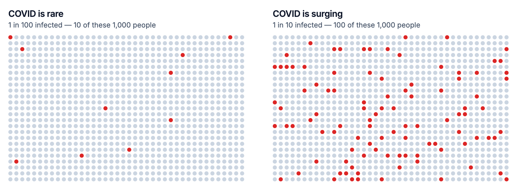
When 1 in 100 is infected, a positive test means a 15 to 20% chance you are infected. When 1 in 10 is infected, the same positive result means around 70%. Built from the numbers in Chapter 6.
Slide 5
Your conclusion depends on what you believed before the evidence
Not the test. Not your result
What changed is what was true before you took the test
That is the prior probability
Slide 6
From diagnosis to data analysis
The same logic applies to a clinical trial
The question becomes: what is the treatment effect?
The test result becomes: the trial data
Disease prevalence becomes: what effect sizes are plausible before we look
Slide 7
The Frequentist approach has no formal role for prior beliefs
You collect data and calculate a p-value
You ask how surprising these data would be if the null hypothesis were true
Prior knowledge might inform your design, but it does not enter the analysis
Slide 8
The Bayesian approach explicitly combines three things
Prior: what you believed about the treatment effect before collecting data
Likelihood: how well different effect sizes explain the data you observed
Posterior: your updated belief after seeing the data
Slide 9
The same data can lead to different conclusions
Start skeptical, see modest evidence, and you might remain unconvinced
Start open-minded and the same evidence might shift your beliefs substantially
It formalizes something we do naturally: extraordinary claims require extraordinary evidence
Slide 10
Re-analyzing the trial
A weakly informative prior
A normal distribution centered at zero, with a standard deviation of 10
The most likely effect is zero, but effects from about -20 to +20 are plausible
Effects larger than that are almost impossible
Slide 11
Open-minded, but not absurd
A prior centered at zero with wide spread lets the data dominate the analysis
While ruling out implausible extremes, like a 50-point improvement on a 63-point scale
With strong prior evidence from previous trials, we might center the prior elsewhere
Slide 12
The same data, analyzed two ways
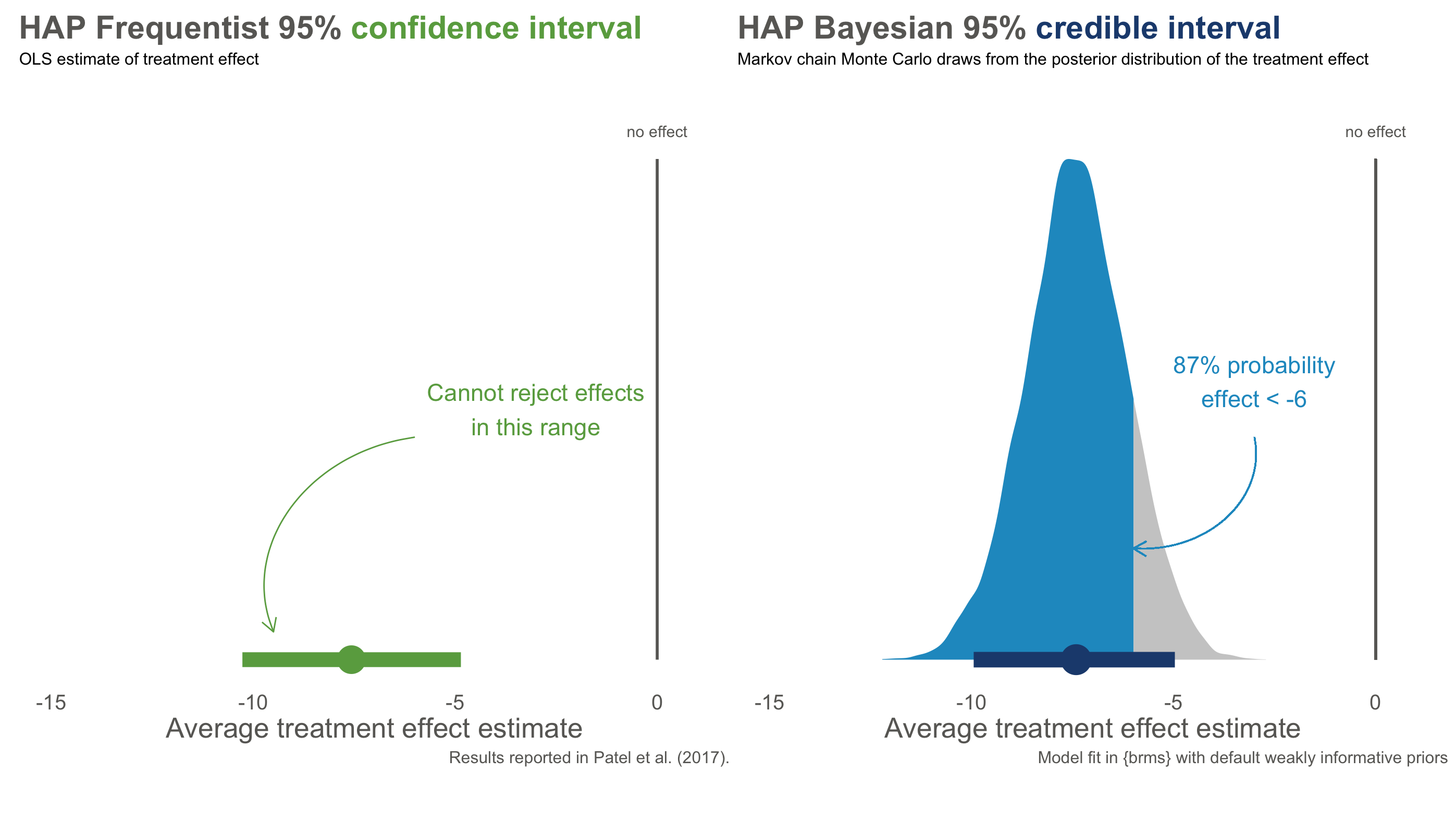
Bayesian re-analysis of the HAP primary outcome of depression severity, against the Frequentist 95% confidence interval. Anonymized data provided by the authors. Reproduced from Chapter 6.
Slide 13
Nearly identical numbers, fundamentally different interpretation
95% confidence interval
A statement about long-run procedures
95% would contain the true effect
It says nothing about this specific interval
95% credible interval
A direct probability statement
95% probability the true effect is in here
Given the data and our prior beliefs
Slide 14
A posterior answers questions a p-value cannot
What's the probability that the effect is larger than -5 points? About 87%
What's the probability of any effect at all, less than zero? Over 99%
These are direct answers to the questions we actually care about
Slide 15
Why not always use Bayesian methods?
Partly history, and partly a genuine tension
Frequentist methods became embedded in training, software, and journal expectations
The computational demands of Bayesian methods were prohibitive until recently
Critics worry that priors introduce subjectivity
Slide 16
Frequentist methods have hidden subjective choices too
Why an alpha of 0.05? Why this particular test?
Making prior assumptions explicit is more honest than pretending they don't exist
With large samples and weak priors, the two approaches often converge — as they did here
Slide 17
Closing reflection
Three things I hope you take away
Report effect sizes, not just p-values
Understand what your intervals mean — one describes a procedure, one describes a belief
Be honest about uncertainty. No statistical test proves a hypothesis true or false
Slide 18
In Closing
A 30% reduction in cancer risk, dismissed because p = 0.06
The authors concluded "no effect" when the data were genuinely ambiguous
Even if we get inference right, we have not asked whether the supplement caused it
Or whether the effect would hold in other populations
Slide 19
The chapter has more than these five videos could carry
Why a 5% false positive rate doesn't mean 5% of significant findings are wrong
Where the smooth bell curve in your stats textbook comes from
What a 7.57-point improvement means clinically, and what it cost per point
The Bayesian approach
Slide 1This is the last video in the chapter. We've spent four videos inside the Frequentist approach, and we ended the last one at its limit: a confidence interval still can't tell you the probability that your hypothesis is correct. The Bayesian approach can. It starts somewhere that might surprise you — with a rapid test.
A positive rapid test, early in the pandemic
COVID is still rare in your community — maybe 1 in 100 people are infected
The test is accurate about 95% of the time
What's the chance you actually have COVID?
Slide 2Imagine it's early in the pandemic. COVID is still rare in your community. Maybe 1 in 100 people are infected. You take a rapid test and it comes back positive. The test is accurate about 95% of the time. What's the chance you actually have COVID?
Most people say 95%. That's not quite right
When the disease is rare, most positive tests are actually false positives
Test 1,000 people, only 10 truly infected, and the test still flags some of the 990
Your actual chance might be closer to 15 to 20%
Slide 3Most people say 95%. But that's not quite right. When the disease is rare, most positive tests are actually false positives. Think about it. If you test 1,000 people and only 10 are truly infected, even a highly accurate test will flag some of the 990 healthy people by mistake. In this scenario, your actual chance of being infected might be closer to 15 or 20%, not 95%.
Same test, same positive result, two months apart
When 1 in 100 is infected, a positive test means a 15 to 20% chance you are infected. When 1 in 10 is infected, the same positive result means around 70%. Built from the numbers in Chapter 6.
Slide 4Here are those two worlds side by side, a thousand people in each. On the left, COVID is rare. 1 in 100 infected, so 10 of these 1,000 people. Now imagine a month later. The virus is surging. 1 in 10 people are infected, which is 100 of them. Same test, same positive result. On the left, your chance of actually being infected if testing positive is 15 or 20%. On the right, it jumps to around 70%.
Your conclusion depends on what you believed before the evidence
Not the test. Not your result
What changed is what was true before you took the test
That is the prior probability
Slide 5What changed? Not the test. Not your result. Just what was true before you took the test — the prior probability. When COVID was rare, a positive result was likely to be wrong. When COVID was common, the same positive result was likely to be right. This is Bayesian reasoning in a nutshell: your conclusion depends on what you believed before you saw the evidence.
From diagnosis to data analysis
The same logic applies to a clinical trial
The question becomes: what is the treatment effect?
The test result becomes: the trial data
Disease prevalence becomes: what effect sizes are plausible before we look
Slide 6The COVID example involves a yes or no question. Am I infected? But the same logic applies when we analyze data from a clinical trial. Instead of asking do I have COVID, we're asking what is the treatment effect. Instead of a test result, we have trial data. And instead of disease prevalence, our prior belief is about what effect sizes are plausible before we see the data.
The Frequentist approach has no formal role for prior beliefs
You collect data and calculate a p-value
You ask how surprising these data would be if the null hypothesis were true
Prior knowledge might inform your design, but it does not enter the analysis
Slide 7In the Frequentist approach we covered earlier, there's no formal role for prior beliefs. You collect data, calculate a p-value, and ask how surprising these data would be if the null hypothesis were true. Your prior knowledge might inform your study design, but it doesn't enter the statistical analysis itself.
The Bayesian approach explicitly combines three things
Prior: what you believed about the treatment effect before collecting data
Likelihood: how well different effect sizes explain the data you observed
Posterior: your updated belief after seeing the data
Slide 8The Bayesian approach is different. It explicitly combines three things. The prior: what you believed about the treatment effect before collecting data. This might be a broad, open-minded prior, or a more skeptical one. The likelihood: how well different effect sizes explain the data you actually observed. This is similar to what Frequentist methods calculate. It's the information in your data. And the posterior: your updated belief after seeing the data, combining your prior belief with the evidence, weighted by how informative each is.
The same data can lead to different conclusions
Start skeptical, see modest evidence, and you might remain unconvinced
Start open-minded and the same evidence might shift your beliefs substantially
It formalizes something we do naturally: extraordinary claims require extraordinary evidence
Slide 9The key insight is that the same data can lead to different conclusions depending on your prior. If you start skeptical and see modest evidence, you might remain unconvinced. If you start open-minded, the same evidence might shift your beliefs substantially. This isn't a bug, it's a feature. It formalizes something we do naturally: extraordinary claims require extraordinary evidence.
Re-analyzing the trial
A weakly informative prior
A normal distribution centered at zero, with a standard deviation of 10
The most likely effect is zero, but effects from about -20 to +20 are plausible
Effects larger than that are almost impossible
Slide 10Let's return to the depression trial to see what this looks like in practice. To run a Bayesian analysis, we first need to specify a prior. What we believe about the treatment effect before seeing the trial data. I used a weakly informative prior: a normal distribution centered at zero with a standard deviation of 10. What does this mean in plain terms? It says: before seeing the data, I think the most likely effect is zero, no difference between groups, but I'm open to effects anywhere from about negative 20 to positive 20 on the depression scale. Effects larger than that are almost impossible.
Open-minded, but not absurd
A prior centered at zero with wide spread lets the data dominate the analysis
While ruling out implausible extremes, like a 50-point improvement on a 63-point scale
With strong prior evidence from previous trials, we might center the prior elsewhere
Slide 11This is a common choice when you want to be open-minded but not absurd. A prior centered at zero with wide spread lets the data dominate the analysis, while ruling out implausible extremes, like an improvement of 50 points on a scale that runs to 63. If we had strong prior evidence from previous trials, we might center the prior elsewhere.
The same data, analyzed two ways
Bayesian re-analysis of the HAP primary outcome of depression severity, against the Frequentist 95% confidence interval. Anonymized data provided by the authors. Reproduced from Chapter 6.
Slide 12This figure compares the Frequentist 95% confidence interval reported in the trial to the Bayesian 95% credible interval, using this prior and the same trial data.
Nearly identical numbers, fundamentally different interpretation
95% confidence interval
A statement about long-run procedures
95% would contain the true effect
It says nothing about this specific interval
95% credible interval
A direct probability statement
95% probability the true effect is in here
Given the data and our prior beliefs
Slide 13The numbers are nearly identical. Both approaches estimate an effect around negative 7.6 points, with similar ranges of uncertainty. But the interpretation is fundamentally different. The confidence interval on the left is a Frequentist statement about long-run procedures. If we repeated this trial many times and calculated intervals each time, 95% of them would contain the true effect. It says nothing about this specific interval. Maybe the true effect is in there, maybe it isn't. We can't assign a probability. The credible interval on the right is a direct probability statement. Given the data and our prior beliefs, there is a 95% probability that the true treatment effect falls in this interval. We can make claims about this specific interval because we're describing our state of knowledge.
A posterior answers questions a p-value cannot
What's the probability that the effect is larger than -5 points? About 87%
What's the probability of any effect at all, less than zero? Over 99%
These are direct answers to the questions we actually care about
Slide 14Even more useful: with a posterior distribution, we can answer questions that Frequentist methods cannot. What's the probability that the effect is larger than negative 5 points? About 87%. What's the probability of any effect at all, less than zero? Over 99%. These are direct answers to the questions we actually care about.
Why not always use Bayesian methods?
Partly history, and partly a genuine tension
Frequentist methods became embedded in training, software, and journal expectations
The computational demands of Bayesian methods were prohibitive until recently
Critics worry that priors introduce subjectivity
Slide 15So if Bayesian methods give us what we want, the probability of hypotheses given data, why doesn't everyone use them? Partly, it's historical. Frequentist methods dominated twentieth-century statistics and became embedded in training, software, and journal expectations. The computational demands of Bayesian methods were also prohibitive until recently. But there are also genuine tensions. Critics worry that priors introduce subjectivity. Two researchers with different priors could reach different conclusions from the same data.
Frequentist methods have hidden subjective choices too
Why an alpha of 0.05? Why this particular test?
Making prior assumptions explicit is more honest than pretending they don't exist
With large samples and weak priors, the two approaches often converge — as they did here
Slide 16Bayesians counter that Frequentist methods have hidden subjective choices too. Why an alpha of 0.05? Why this particular test? And that making prior assumptions explicit is more honest than pretending they don't exist. In practice, when sample sizes are large and priors are weak, Frequentist and Bayesian answers often converge, as they did in this trial. The differences matter most when data are sparse, priors are strong, or you need to make direct probability statements about hypotheses.
Closing reflection
Three things I hope you take away
Report effect sizes, not just p-values
Understand what your intervals mean — one describes a procedure, one describes a belief
Be honest about uncertainty. No statistical test proves a hypothesis true or false
Slide 17Statistical inference is hard. Don't be discouraged if these concepts require multiple readings and practice to internalize. Even experienced researchers misinterpret p-values and confidence intervals. Here's what I hope you take away. Report effect sizes, not just p-values. A p-value tells you whether a result is surprising under the null hypothesis, nothing more. Understand what your intervals mean. A 95% confidence interval is a statement about a procedure. A 95% credible interval is a statement about that specific interval, but it depends on your prior. Neither is right; they answer different questions. And be honest about uncertainty. No statistical test proves a hypothesis true or false.
In Closing
A 30% reduction in cancer risk, dismissed because p = 0.06
The authors concluded "no effect" when the data were genuinely ambiguous
Even if we get inference right, we have not asked whether the supplement caused it
Or whether the effect would hold in other populations
Slide 18Think back to where we started: a vitamin D trial where a 30% reduction in cancer risk was dismissed because the p-value was 0.06. The authors concluded no effect when the data were genuinely ambiguous. That's a threat to statistical conclusion validity, drawing the wrong conclusion from the evidence. But even if we get inference right, even if we correctly conclude the supplement probably reduces cancer risk, we still haven't answered whether it causes that reduction, or whether the effect would hold in other populations. Those are questions of internal and external validity, and they're where we turn next.
The chapter has more than these five videos could carry
Why a 5% false positive rate doesn't mean 5% of significant findings are wrong
Where the smooth bell curve in your stats textbook comes from
What a 7.57-point improvement means clinically, and what it cost per point
Slide 19One last thing. These five videos carry the spine of the chapter, but the chapter carries more. Go read it for the parts we left on the page. Why controlling your false positive rate at 5% does not mean that 5% of significant findings are wrong. Where the smooth bell curve in your statistics textbook comes from, and how it relates to the simulation we ran. And what an improvement of 7.57 points on the depression scale actually means clinically, including what it cost per point. The chapter has all of it, with the references.