Chapter 7 · Video 2
The road not taken
Print layout
Slide 1


The road not taken
Slide 2
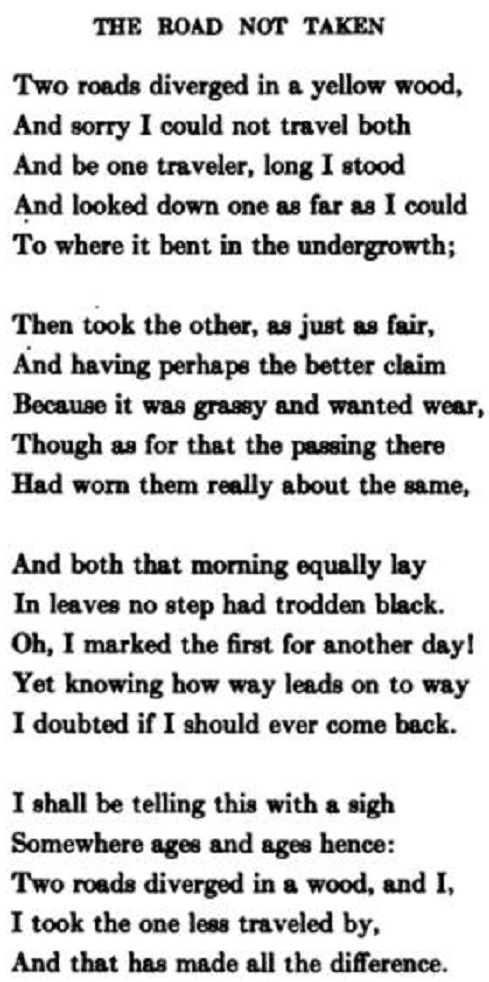
The Road Not Taken. Reproduced from Chapter 7.
Two roads diverged in a yellow wood
What did happen
What would have happened
Slide 3
Robert has to choose one road; he can't take both
X = 0 — the road more traveled
X = 1 — the road less traveled
Slide 4
Why X and Y, and why 1 and 0?
Potential causes are X; response variables are Y
A treatment or exposure with two levels: treated 1, not treated 0
Slide 5
The road less traveled is the treatment: X = 1
"Grassy and wanted wear" — so he went right
"And that has made all the difference"
Slide 6
Rubin, 1974
Two roads, two potential outcomes
Y if X = 0 — what happens on the road more traveled
Y if X = 1 — what happens on the road less traveled
Slide 7
One outcome becomes fact; the other becomes counterfactual
He takes the road less traveled, and that outcome is observed
The road more traveled is never observed for him
Slide 8
How can he know that it made all the difference?
A causal effect is the difference between what did and would have happened
We observed only what did happen
A missing data problem
Slide 9
Holland, 1986
The fundamental problem of causal inference
We observe one potential outcome per person, or per unit
An individual causal effect needs both of them
So it cannot be measured for Robert
Slide 10
We estimate the average treatment effect
Truly calculating it would need both potential outcomes for everyone
Units can be people, or classrooms, or schools
We observe one outcome per unit, so the ATE is estimated
Slide 11
Each traveler has two happiness scores, one for each road
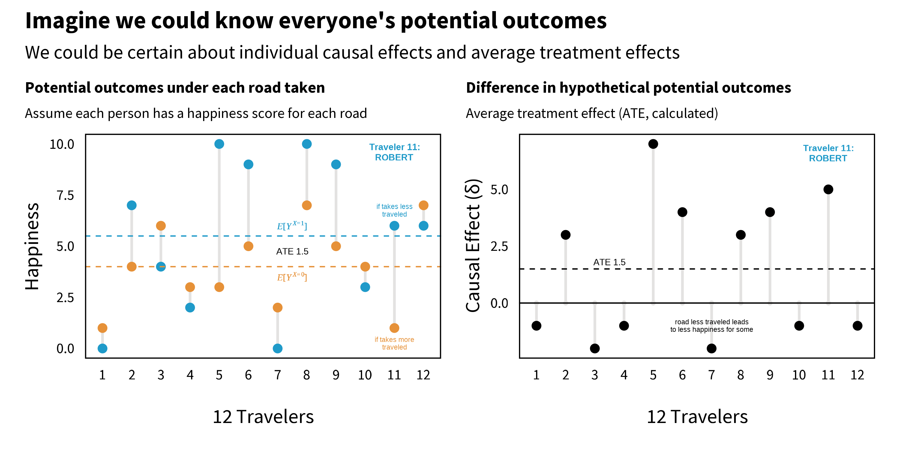
Potential outcomes, part 1. Fictional happiness data for twelve travelers under both roads, on a scale of 0 to 10. Reproduced from Chapter 7.
Slide 12
The true ATE is 1.5 points of happiness
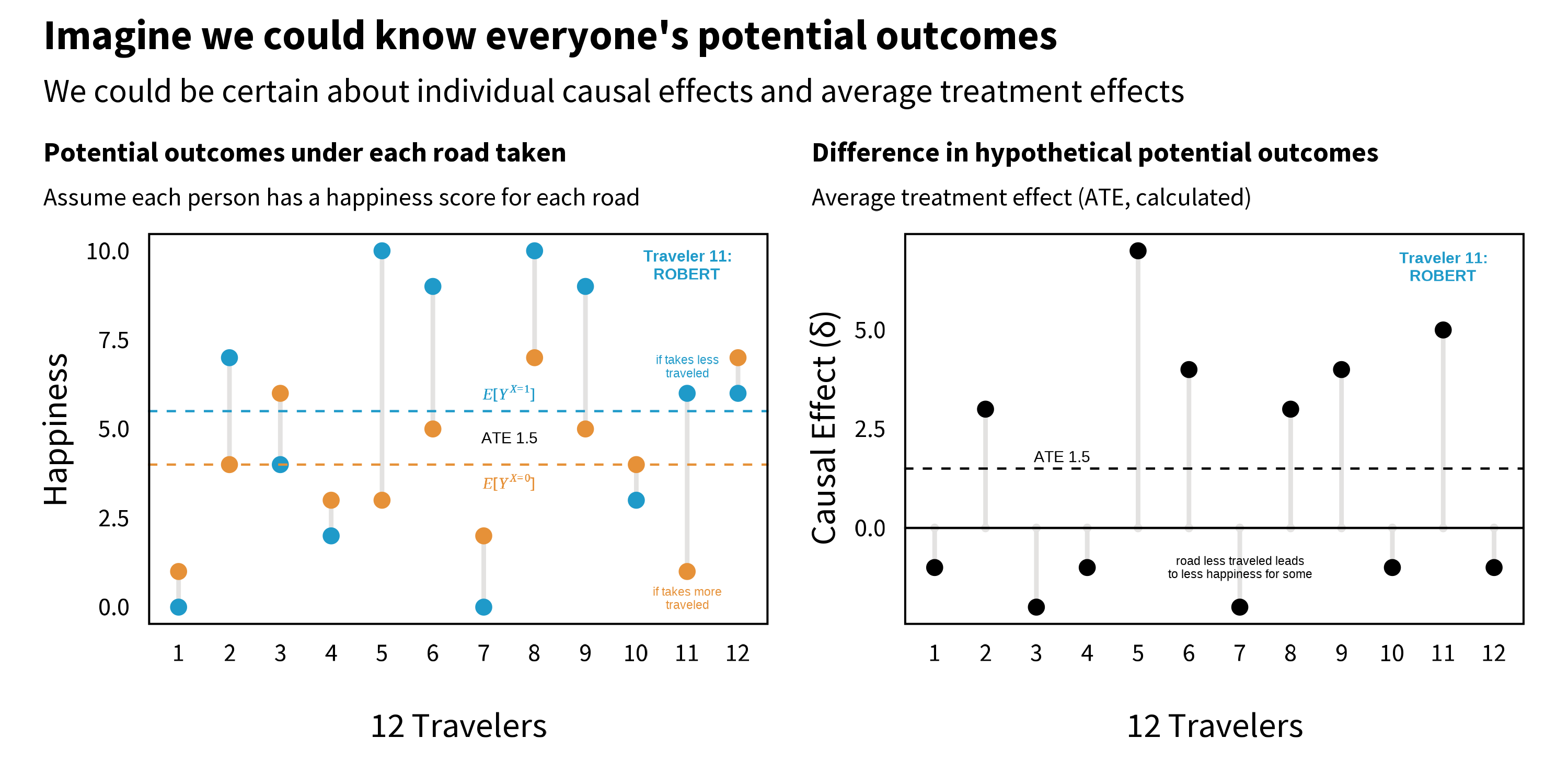
Right panel: each traveler's individual causal effect, and their average. Some travelers are made worse off by the road less traveled. Reproduced from Chapter 7.
Slide 13
How do people come to take one road versus the other?
We compare those who took one road to those who took the other
Two scenarios, out of an infinite number
Slide 14
A. Travelers are randomly assigned, and the estimate is 1.5
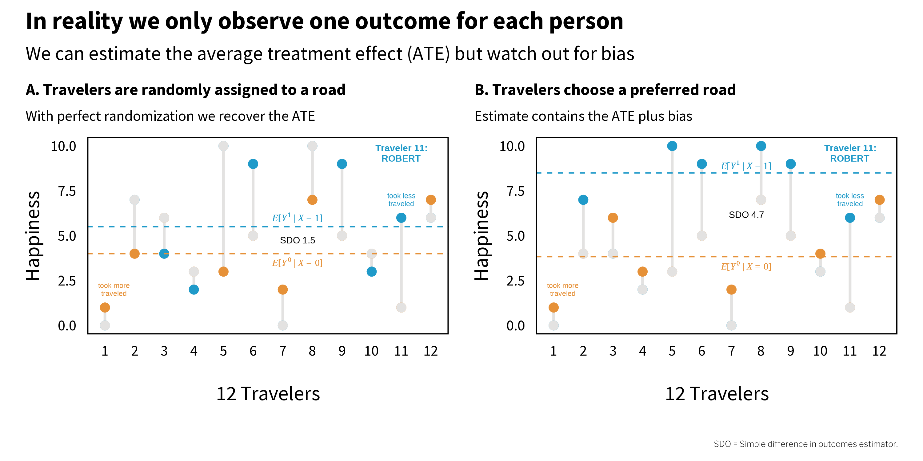
Potential outcomes, part 2. Grey dots are the unobserved counterfactuals. Under perfect randomization the estimate equals the true ATE. Reproduced from Chapter 7.
Slide 15
B. Travelers choose a road, and the estimate is 4.7
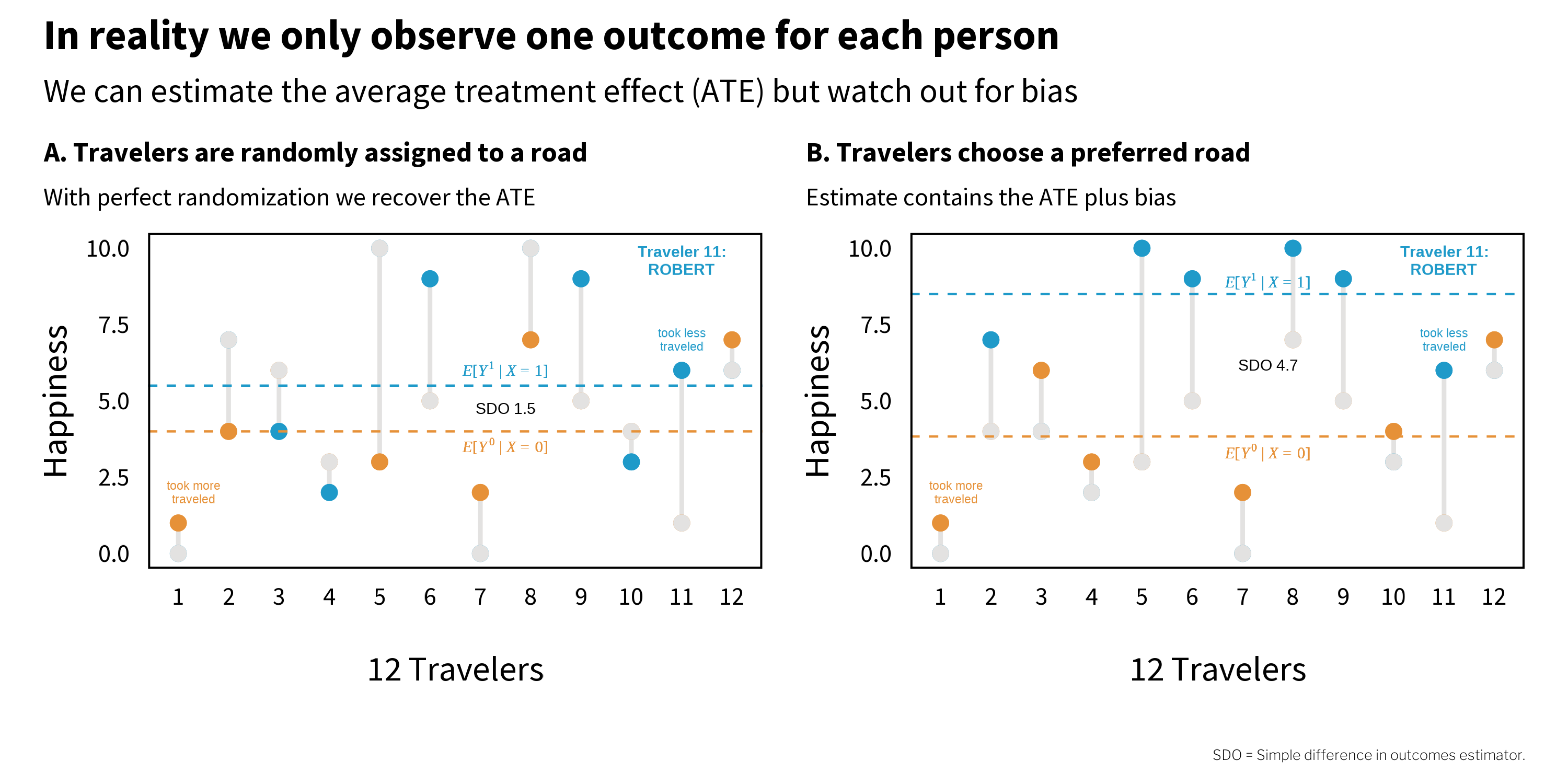
Panel B. The same twelve travelers, each picking the road that maximizes their own happiness. The estimate now contains the ATE plus bias. Reproduced from Chapter 7.
Slide 16
Selection bias: systematic differences that distort the comparison
Optimists would have been happier on either road
They selected into the road less traveled
The comparison now carries the road and the optimism together
Slide 17
Randomization neutralizes selection bias where it is available
Most research is non-experimental, or observational
The size of the bias is typically unknowable, so it can't be subtracted away
Research design and statistical adjustment are the defense
Slide 18
Cunningham, 2021
The entire enterprise of causal inference is about negating selection bias
That is the problem every method in this chapter is built to solve
Slide 19
Which approach depends on context and discipline
Experimental
Randomly allocate units to arms
Clinical trialists and policy scholars
Applied in development economics
Non-experimental
Randomization is not available
Rooted in observational data
Slide 20
Matthay et al., 2020
Two families of non-experimental approaches
Confounder-control
Statistical adjustment for comparability
Common in epidemiology and public health
Instrument-based
Leverage arbitrary reasons for treatment
Also called quasi-experimental designs
Common in economics and psychology
Slide 21
In Closing
Both families answer the same problem: selection bias
Confounder-control adjusts statistically to make groups more comparable
Instrument-based designs find arbitrary reasons for being treated
The chapter takes each in turn, and so do the videos that follow
The road not taken
Slide 1Causal inference is an exercise in counterfactual thinking, full of what if questions about the road not taken. We ask ourselves these questions all the time. What would have happened if I had taken that job? Said yes instead of no? How would life be different today?
The Road Not Taken. Reproduced from Chapter 7.
Two roads diverged in a yellow wood
What did happen
What would have happened
Slide 2A counterfactual is the hypothetical state of a what if question. With counterfactual thinking, there is what actually happened, and then there is the hypothetical counterfactual of what would have happened, counter to fact, under the alternative scenario. The difference between what did happen and what would have happened is known as the causal effect. Robert Frost fans see the problem. Two roads diverged in a yellow wood, and sorry I could not travel both and be one traveler.
Robert has to choose one road; he can't take both
X = 0 — the road more traveled
X = 1 — the road less traveled
Slide 3Robert has to choose one road. He can't take both simultaneously. He can either take the road more traveled, a decision we'll call X equals zero, or he can take the road less traveled, a decision we'll call X equals one.
Why X and Y, and why 1 and 0?
Potential causes are X; response variables are Y
A treatment or exposure with two levels: treated 1, not treated 0
Slide 4In some ways it might be easier to refer to Robert's decision as the variable road, or R, and set the values of road to more traveled or less traveled, representing his two choices. But instead I'm referring to his decision as X, and to the values of X as zero and one. Why? Often we refer to potential causes as X and to response variables as Y. And typically, when the treatment, or exposure, X can take two levels, such as treated and not treated, we label treated one, and not treated zero.
The road less traveled is the treatment: X = 1
"Grassy and wanted wear" — so he went right
"And that has made all the difference"
Slide 5In this example, I imagine Robert looking left and then looking right. Observing that the second path was grassy and wanted wear, he decided to go right, taking the one less traveled by. Frost claims that his decision to take the uncommon path made all the difference, so I'm labeling that path, the road less traveled, as the treatment. X equals one.
Rubin, 1974
Two roads, two potential outcomes
Y if X = 0 — what happens on the road more traveled
Y if X = 1 — what happens on the road less traveled
Slide 6Robert's two choices correspond to two potential outcomes, or states of the world, that he could experience. There is the potential outcome that results from taking the road more traveled, and the potential outcome that results from taking the road less traveled. We'll call these Y if X equals zero, what happens if he takes the road more traveled, and Y if X equals one, what happens if he takes the road less traveled.
One outcome becomes fact; the other becomes counterfactual
He takes the road less traveled, and that outcome is observed
The road more traveled is never observed for him
Slide 7So what does he do? He famously takes the road less traveled. Robert's factual outcome is what happens after making that choice. His other potential outcome will never be observed. Taking the road more traveled is now the counterfactual. He can only wonder what would have happened, counter to fact, if he had taken the beaten path.
How can he know that it made all the difference?
A causal effect is the difference between what did and would have happened
We observed only what did happen
A missing data problem
Slide 8And yet, Robert boldly claims that taking the road less traveled made all the difference. How can he know for sure? We defined causal effects as the difference between what did happen and what would have happened, but we only observed what happened, not what would have. So we have a missing data problem.
Holland, 1986
The fundamental problem of causal inference
We observe one potential outcome per person, or per unit
An individual causal effect needs both of them
So it cannot be measured for Robert
Slide 9This is what's often called the fundamental problem of causal inference. We only get to observe one potential outcome for any given person, or unit, more generally. The causal effect of taking the road less traveled is the difference in the two potential outcomes, Y if X equals one minus Y if X equals zero. But Y if X equals zero is missing. So we can't measure this effect for Robert.
We estimate the average treatment effect
Truly calculating it would need both potential outcomes for everyone
Units can be people, or classrooms, or schools
We observe one outcome per unit, so the ATE is estimated
Slide 10We can, however, compare groups of people like Robert who take one road or the other and estimate the average treatment effect, or A T E. I'm emphasizing estimate, because truly calculating the average treatment effect would require knowing both potential outcomes for each person, or unit, like classrooms or schools. We can only observe one potential outcome for any given person. But let's ignore that for a moment, to understand the true average treatment effect.
Each traveler has two happiness scores, one for each road
Potential outcomes, part 1. Fictional happiness data for twelve travelers under both roads, on a scale of 0 to 10. Reproduced from Chapter 7.
Slide 11While we're pretending, let's imagine that the response variable Robert writes about in his poem is happiness later in life, and happiness, our Y, is measured on a scale of zero to ten, where zero is not at all happy and ten is very happy. The left panel here shows fictional happiness data for a sample of twelve people, including Robert, under both potential outcomes. Notice how each person has two values: the happiness that would result if they took the road less traveled, and the happiness that would result if they took the road more traveled. Some people, like the first traveler on the left, would be happiest taking the road more traveled. Other people, such as Robert, who is number eleven, would find greater happiness on the road less traveled.
The true ATE is 1.5 points of happiness
Right panel: each traveler's individual causal effect, and their average. Some travelers are made worse off by the road less traveled. Reproduced from Chapter 7.
Slide 12As shown in the right panel, the average treatment effect is calculated as the difference between the group averages, which is equivalent to the average of the travelers' individual causal effects. In this example, where we are all knowing, the average treatment effect is one point five. Taking the road less traveled increases happiness on average by one point five points on a scale of zero to ten. Remember, we're pretending here. We never observe both potential outcomes.
How do people come to take one road versus the other?
We compare those who took one road to those who took the other
Two scenarios, out of an infinite number
Slide 13We're not all knowing, of course, and we only get to observe one potential outcome for each person. This means we have to estimate the average treatment effect by comparing people like Robert who take the road less traveled to people who take the road more traveled. But how do people come to take one road versus the other?
A. Travelers are randomly assigned, and the estimate is 1.5
Potential outcomes, part 2. Grey dots are the unobserved counterfactuals. Under perfect randomization the estimate equals the true ATE. Reproduced from Chapter 7.
Slide 14This figure shows two scenarios, of an infinite number. On the left, in panel A, travelers are randomly assigned to a road. Imagine that they come to the fork in the road and pull directions out of a hat. Half are assigned to the road less traveled, and half to the road more traveled. In both panels, the grey dots represent the unobserved counterfactuals. Notice that under perfect randomization, on the left, the estimated average treatment effect of one point five is equal to the true, but unknowable, average treatment effect.
B. Travelers choose a road, and the estimate is 4.7
Panel B. The same twelve travelers, each picking the road that maximizes their own happiness. The estimate now contains the ATE plus bias. Reproduced from Chapter 7.
Slide 15On the right, in panel B, travelers choose a road themselves. Imagine that they go with their gut and all happen to pick the road that maximizes their individual happiness. Here the estimate is four point seven. That does not line up with the true average treatment effect, because the estimate includes bias. And remember that bias is anything that takes us away from the truth.
Selection bias: systematic differences that distort the comparison
Optimists would have been happier on either road
They selected into the road less traveled
The comparison now carries the road and the optimism together
Slide 16Why does the estimate go wrong in panel B? The answer is selection bias, systematic differences between groups that distort our comparison. When travelers chose their own road, the optimistic people, who would have been happier regardless of which road they took, selected into the road less traveled. So when we compare average happiness across roads, we're not just seeing the effect of the road. We're also seeing the effect of optimism.
Randomization neutralizes selection bias where it is available
Most research is non-experimental, or observational
The size of the bias is typically unknowable, so it can't be subtracted away
Research design and statistical adjustment are the defense
Slide 17As we will see in later chapters, randomization can be a very effective way to neutralize selection bias, but randomization is not always possible or maintained. Most research is non-experimental, or what many would call observational. Selection bias will remain a threat in many cases, and unfortunately we can't simply calculate it and subtract it away, because the exact quantity is typically unknowable. That leaves us with research design and statistical adjustment as our only defense.
Cunningham, 2021
The entire enterprise of causal inference is about negating selection bias
That is the problem every method in this chapter is built to solve
Slide 18Cunningham has argued that the entire enterprise of causal inference is about developing a reasonable strategy for negating the role that selection bias is playing in estimated causal effects.
Which approach depends on context and discipline
Experimental
Randomly allocate units to arms
Clinical trialists and policy scholars
Applied in development economics
Non-experimental
Randomization is not available
Rooted in observational data
Slide 19There are different causal inference methods for addressing selection bias, and which one a researcher chooses tends to be heavily influenced by their context and discipline. Clinical researchers, biostatisticians, and behavioral interventionists often prefer to use experimental designs that randomly allocate people, or units, to different treatment arms. Folks in this camp might refer to themselves as clinical trialists. There is also a rich tradition of experimentation in the social sector among economists and public policy scholars. Three economists won the twenty nineteen Nobel Prize in Economics for their experimental approach to alleviating global poverty. Where randomization is not available, the work has to be non-experimental.
Matthay et al., 2020
Two families of non-experimental approaches
Confounder-control
Statistical adjustment for comparability
Common in epidemiology and public health
Instrument-based
Leverage arbitrary reasons for treatment
Also called quasi-experimental designs
Common in economics and psychology
Slide 20Many research questions in global health are not amenable to experimentation, and the approach to causal inference must be rooted in non-experimental, or observational, data. These non-experimental approaches divide into two main buckets: confounder-control and instrument-based. Confounder-control is characterized by the use of statistical adjustment to make groups more comparable. You'll find many examples of confounder-control in epidemiology and public health journals. Instrument-based studies, sometimes called quasi-experimental designs, estimate treatment effects by finding and leveraging arbitrary reasons why some people are more likely to be treated or exposed. Instrument-based studies are quite common in economics and psychology.
In Closing
Both families answer the same problem: selection bias
Confounder-control adjusts statistically to make groups more comparable
Instrument-based designs find arbitrary reasons for being treated
The chapter takes each in turn, and so do the videos that follow
Slide 21Both families of approaches exist to answer the same problem. Confounder-control uses statistical adjustment to make groups more comparable. Instrument-based studies find and leverage arbitrary reasons why some people are more likely to be treated. The chapter introduces each approach in turn, and so do the videos that follow.